P1
You are given the file points.mat with training data. There are three kinds of points. The goal is to train with these data and classify the points in . Modify the file netbpfull.m such that it works with the three categories of points.
• Load the data with load points.mat. This will result in an array containing points
in 2D and an array labels containing labels.
• Modify the function cost such that it returns
and also returns the indices (in x) of training points that are not classified correctly.
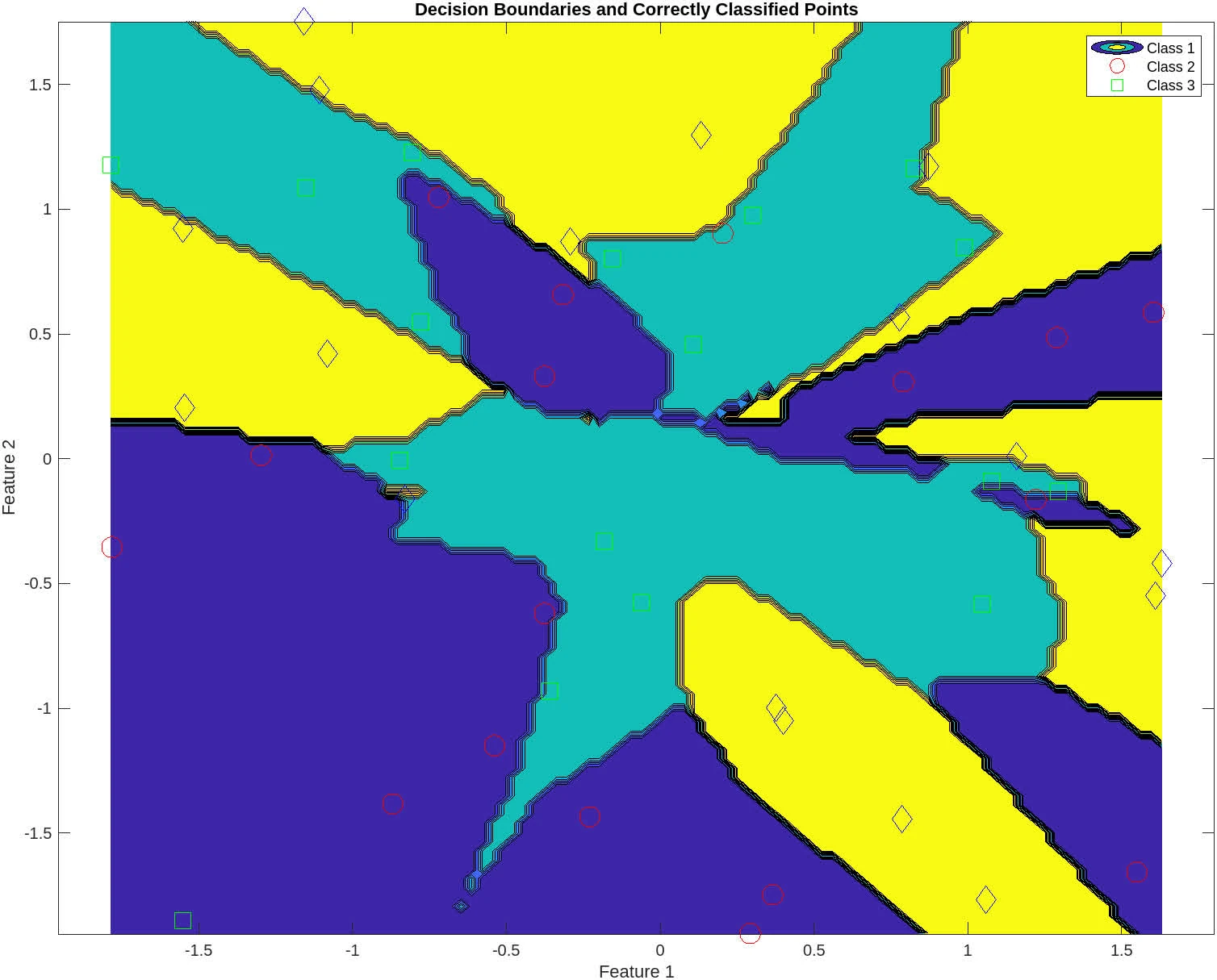
• netbpfull.m should plot
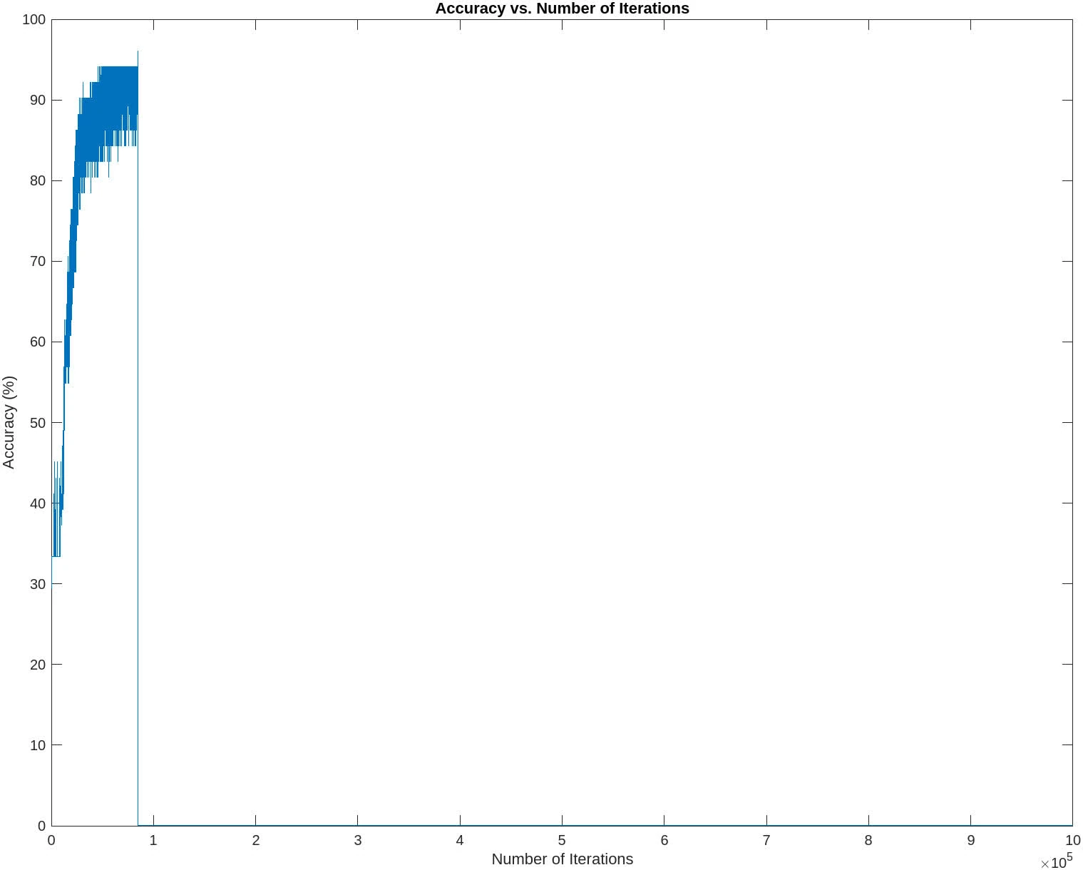
- accuracy versus number of iterations
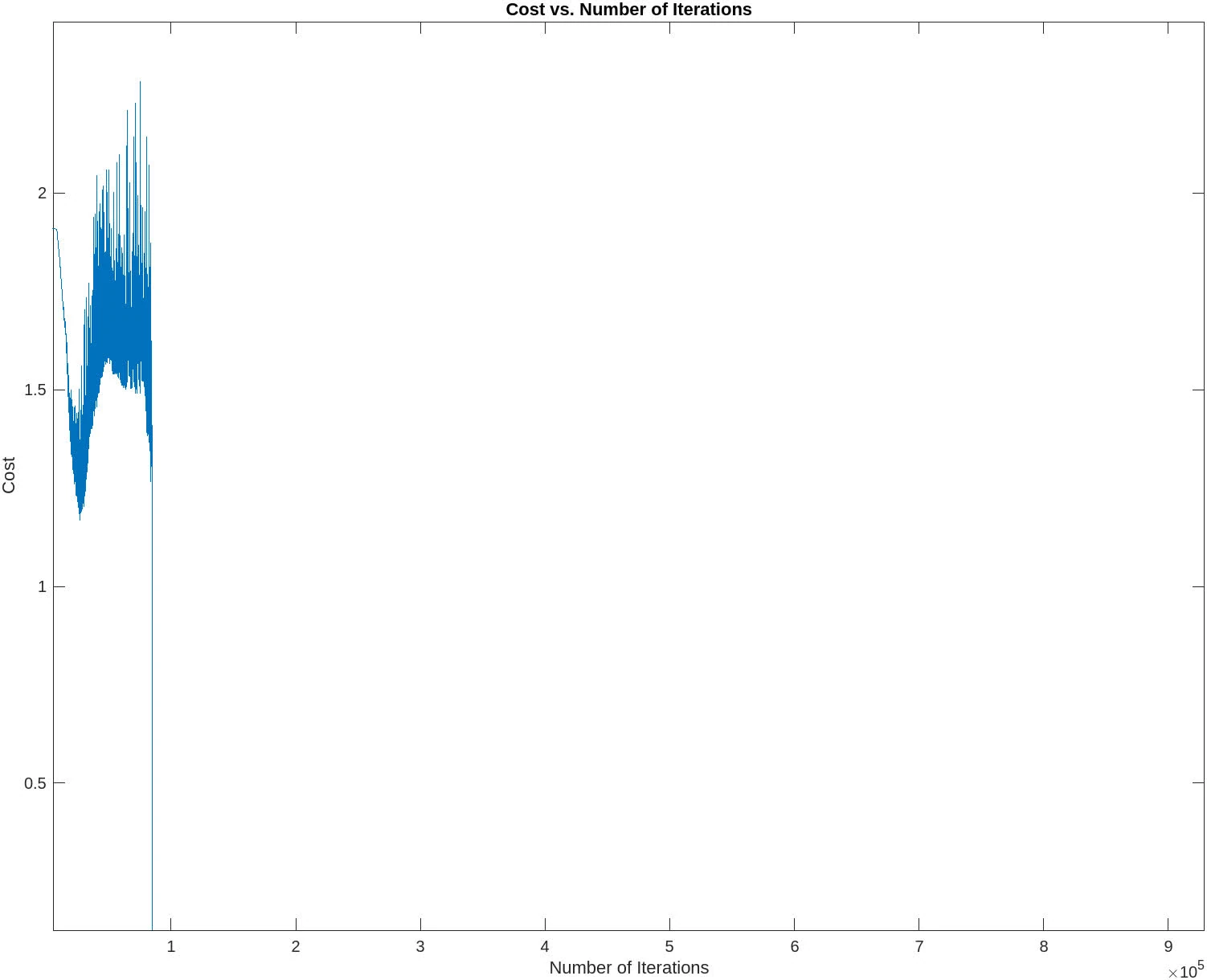
- cost versus number of iterations and
- two plots like in
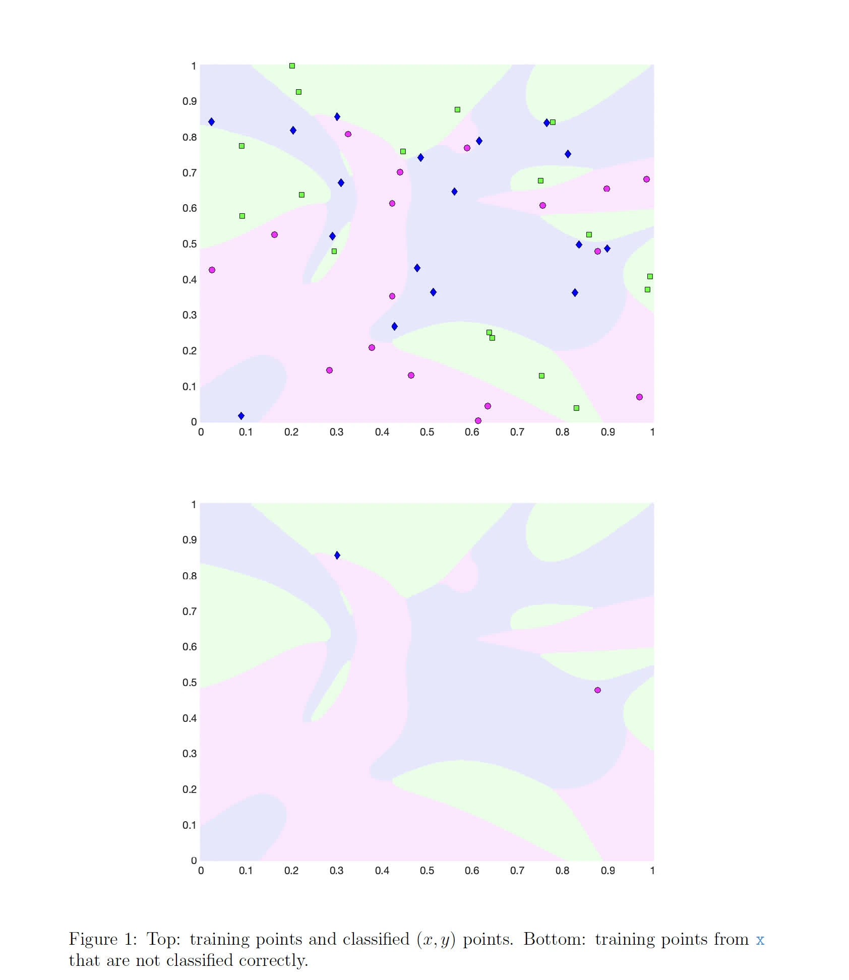
figure1: this plot - The training should stop if accuracy of 95% is reached; otherwise it should continue to
Niter=1e6. For full marks, you need to achieve 95%.
For pretty code, see net.py.
Solution
The following contains the diff of the original netbpfull.m and the modified version
diff --git a/content/thoughts/university/compsci-4x03/netbpfull.m b/content/thoughts/university/compsci-4x03/netbpfull.m
index 5a1b6e13..df3714f9 100644
--- a/content/thoughts/university/compsci-4x03/netbpfull.m
+++ b/content/thoughts/university/compsci-4x03/netbpfull.m
@@ -1,134 +1,225 @@
 function netbp_full
 %NETBP_FULL
 %   Extended version of netbp, with more graphics
-%
-%   Set up data for neural net test
-%   Use backpropagation to train
-%   Visualize results
-%
-% C F Higham and D J Higham, Aug 2017
-%
-%
-% xcoords, ycoords, targets
-x1 = [0.1,0.3,0.1,0.6,0.4,0.6,0.5,0.9,0.4,0.7];
-x2 = [0.1,0.4,0.5,0.9,0.2,0.3,0.6,0.2,0.4,0.6];
-y = [ones(1,5) zeros(1,5); zeros(1,5) ones(1,5)];
-
-figure(1)
-clf
-a1 = subplot(1,1,1);
-plot(x1(1:5),x2(1:5),'ro','MarkerSize',12,'LineWidth',4)
-hold on
-plot(x1(6:10),x2(6:10),'bx','MarkerSize',12,'LineWidth',4)
-a1.XTick = [0 1];
-a1.YTick = [0 1];
-a1.FontWeight = 'Bold';
-a1.FontSize = 16;
-xlim([0,1])
-ylim([0,1])
-
-%print -dpng pic_xy.webp
-
-
-% Initialize weights and biases
+
+% Load the data
+load points.mat x; % This loads 'x' which contains points and 'labels'
+load points.mat labels; % This loads 'x' which contains points and 'labels'
+
+x_mean = mean(x, 2);
+x_std = std(x, 0, 2);
+x = (x - x_mean) ./ x_std; % Normalize the data
+
+% Initialize weights and biases for a network with three outputs
 rng(5000);
-W2 = 0.5*randn(2,2);
-W3 = 0.5*randn(3,2);
-W4 = 0.5*randn(2,3);
-b2 = 0.5*randn(2,1);
-b3 = 0.5*randn(3,1);
-b4 = 0.5*randn(2,1);
-
-
-
-% Forward and Back propagate
-% Pick a training point at random
-eta = 0.05;
+num_hidden_1 = 20; % Increased the number of neurons
+num_hidden_2 = 20;
+W2 = randn(num_hidden_1, 2) * 0.01;
+W3 = randn(num_hidden_2, num_hidden_1) * 0.01;
+W4 = randn(size(labels, 1), num_hidden_2) * 0.01;
+b2 = zeros(num_hidden_1, 1);
+b3 = zeros(num_hidden_2, 1);
+b4 = zeros(size(labels, 1), 1);
+
+% Training parameters
+eta = 0.001; % Adjusted learning rate
+alpha = 0.89; % Momentum term
+alpha_leak = 0.01; % Define this once at the beginning of your script
+lambda = 0.001; % L2 Regularization strength
 Niter = 1e6;
-savecost = zeros(Niter,1);
+batch_size = 16; % Adjusted batch size for batch training
+% Learning rate decay
+decay_rate = 0.99;
+decay_step = 10000; % Apply decay every 10000 iterations
+
+% buffers
+savecost = zeros(Niter, 1);
+saveaccuracy = zeros(Niter, 1);
+savemisclassified = cell(Niter, 1);
+
+% Momentum variables
+mW2 = zeros(size(W2));
+mW3 = zeros(size(W3));
+mW4 = zeros(size(W4));
+mb2 = zeros(size(b2));
+mb3 = zeros(size(b3));
+mb4 = zeros(size(b4));
+
+% Training loop with batch training
 for counter = 1:Niter
-    k = randi(10);
-    x = [x1(k); x2(k)];
-    % Forward pass
-    a2 = activate(x,W2,b2);
-    a3 = activate(a2,W3,b3);
-    a4 = activate(a3,W4,b4);
-    % Backward pass
-    delta4 = a4.*(1-a4).*(a4-y(:,k));
-    delta3 = a3.*(1-a3).*(W4'*delta4);
-    delta2 = a2.*(1-a2).*(W3'*delta3);
-    % Gradient step
-    W2 = W2 - eta*delta2*x';
-    W3 = W3 - eta*delta3*a2';
-    W4 = W4 - eta*delta4*a3';
-    b2 = b2 - eta*delta2;
-    b3 = b3 - eta*delta3;
-    b4 = b4 - eta*delta4;
-    % Monitor progress
-    newcost = cost(W2,W3,W4,b2,b3,b4);   % display cost to screen
-    newcost = cost(W2,W3,W4,b2,b3,b4);   % display cost to screen
-    fprintf("iter=% 5d   cost=%e\n", counter, newcost)
+    % Select a batch of points
+    batch_indices = randperm(size(x, 2), batch_size);
+    x_batch = x(:, batch_indices);
+    labels_batch = labels(:, batch_indices);
+
+    % Initialize gradients for the batch
+    gradW2 = zeros(size(W2));
+    gradW3 = zeros(size(W3));
+    gradW4 = zeros(size(W4));
+    gradb2 = zeros(size(b2));
+    gradb3 = zeros(size(b3));
+    gradb4 = zeros(size(b4));
+
+    % Loop over all examples in the batch
+    for k = 1:batch_size
+        xk = x_batch(:, k);
+        labelk = labels_batch(:, k);
+
+        % Forward pass
+        a2 = actfn(xk, W2, b2, 'leaky_relu');
+        a3 = actfn(a2, W3, b3, 'leaky_relu');
+        a4 = actfn(a3, W4, b4, 'sigmoid');
+
+        % Backward pass
+        delta4 = (a4 - labelk) .* a4 .* (1 - a4);
+        delta3 = (W4' * delta4) .* (a3 > 0 + alpha_leak * (a3 <= 0)); % Leaky ReLU derivative
+        delta2 = (W3' * delta3) .* (a2 > 0 + alpha_leak * (a2 <= 0)); % Leaky ReLU derivative
+
+        % Accumulate gradients over the batch
+        gradW4 = gradW4 + delta4 * a3';
+        gradW3 = gradW3 + delta3 * a2';
+        gradW2 = gradW2 + delta2 * xk';
+        gradb4 = gradb4 + delta4;
+        gradb3 = gradb3 + delta3;
+        gradb2 = gradb2 + delta2;
+    end
+
+    % Average gradients over the batch
+    gradW4 = gradW4 + (lambda / batch_size) * W4;
+    gradW3 = gradW3 + (lambda / batch_size) * W3;
+    gradW2 = gradW2 + (lambda / batch_size) * W2;
+    gradb4 = gradb4 / batch_size;
+    gradb3 = gradb3 / batch_size;
+    gradb2 = gradb2 / batch_size;
+
+    % Update weights with gradients
+    mW4 = alpha * mW4 - eta * gradW4;
+    mW3 = alpha * mW3 - eta * gradW3;
+    mW2 = alpha * mW2 - eta * gradW2;
+    mb4 = alpha * mb4 - eta * gradb4;
+    mb3 = alpha * mb3 - eta * gradb3;
+    mb2 = alpha * mb2 - eta * gradb2;
+
+    W4 = W4 + mW4;
+    W3 = W3 + mW3;
+    W2 = W2 + mW2;
+    b4 = b4 + mb4;
+    b3 = b3 + mb3;
+    b2 = b2 + mb2;

+    % Calculate cost and accuracy for the whole dataset
+    [newcost, accuracy, misclassified] = cost(W2, W3, W4, b2, b3, b4, x, labels);
     savecost(counter) = newcost;
+    saveaccuracy(counter) = accuracy;
+    savemisclassified{counter} = misclassified;
+
+    % Apply decay to the learning rate
+    if mod(counter, decay_step) == 0
+        eta = eta * decay_rate;
+    end
+
+    % Early stopping if accuracy is above 95%
+    if accuracy >= 95
+        fprintf('Achieved 95\n', counter, newcost, accuracy);
+    end
 end

-figure(2)
-clf
-semilogy([1:1e4:Niter],savecost(1:1e4:Niter),'b-','LineWidth',2)
-xlabel('Iteration Number')
-ylabel('Value of cost function')
-set(gca,'FontWeight','Bold','FontSize',18)
-print -dpng pic_cost.webp
-
-%%% Display shaded and unshaded regions
-N = 500;
-Dx = 1/N;
-Dy = 1/N;
-xvals = [0:Dx:1];
-yvals = [0:Dy:1];
-for k1 = 1:N+1
-    xk = xvals(k1);
-    for k2 = 1:N+1
-        yk = yvals(k2);
-        xy = [xk;yk];
-        a2 = activate(xy,W2,b2);
-        a3 = activate(a2,W3,b3);
-        a4 = activate(a3,W4,b4);
-        Aval(k2,k1) = a4(1);
-        Bval(k2,k1) = a4(2);
-     end
+% After training loop: Plot accuracy vs. number of iterations
+figure;
+plot(saveaccuracy);
+xlabel('Number of Iterations');
+ylabel('Accuracy (%)');
+title('Accuracy vs. Number of Iterations');
+
+% Plot cost vs. number of iterations
+figure;
+plot(savecost);
+xlabel('Number of Iterations');
+ylabel('Cost');
+title('Cost vs. Number of Iterations');
+
+% Plot decision boundaries and points
+% First, create a meshgrid to cover the input space
+[xv, yv] = meshgrid(linspace(min(x(1,:)), max(x(1,:)), 100), linspace(min(x(2,:)), max(x(2,:)), 100));
+mesh_x = [xv(:)'; yv(:)'];
+mesh_a2 = actfn(mesh_x, W2, b2, 'leaky_relu');
+mesh_a3 = actfn(mesh_a2, W3, b3, 'leaky_relu');
+mesh_a4 = actfn(mesh_a3, W4, b4, 'sigmoid');
+[~, mesh_classes] = max(mesh_a4);
+mesh_classes = reshape(mesh_classes, size(xv));
+
+% Find the misclassified points from the last iteration
+misclassified_indices = savemisclassified{end};
+classified_correctly_indices = setdiff(1:size(x, 2), misclassified_indices);
+
+% First Plot: Decision boundaries and correctly classified points only
+figure;
+contourf(xv, yv, mesh_classes);
+hold on;
+gscatter(x(1,classified_correctly_indices), x(2,classified_correctly_indices), vec2ind(labels(:,classified_correctly_indices)), 'rgb', 'osd', 12, 'LineWidth', 4);
+title('Decision Boundaries and Correctly Classified Points');
+xlabel('Feature 1');
+ylabel('Feature 2');
+legend('Class 1', 'Class 2', 'Class 3');
+hold off;
+
+% Second Plot: Decision boundaries and misclassified points only
+figure;
+contourf(xv, yv, mesh_classes);
+hold on;
+gscatter(x(1,misclassified_indices), x(2,misclassified_indices), vec2ind(labels(:,misclassified_indices)), 'rgb', 'osd', 12, 'LineWidth', 4);
+title('Decision Boundaries and Misclassified Points Only');
+xlabel('Feature 1');
+ylabel('Feature 2');
+legend('Misclassified');
+hold off;
+
+
+% Activation function with switch for ReLU
+function z = actfn(x, W, b, activation_type)
+    if strcmp(activation_type, 'leaky_relu')
+        % Define the Leaky ReLU slope for negative inputs
+        alpha_leak = 0.01;
+        z = max(alpha_leak * (W * x + b), W * x + b);
+    elseif strcmp(activation_type, 'relu')
+        z = max(0, W * x + b);
+    else
+        z = 1 ./ (1 + exp(-W * x - b));
+    end
+end
+
+% Cost function with accuracy and misclassified indices calculation
+function [costval, accuracy, misclassified] = cost(W2, W3, W4, b2, b3, b4, x, labels)
+    misclassified = [];
+    correct_count = 0;
+    costval = 0; % Initialize the cost value
+
+    for i = 1:size(x, 2)
+        input = x(:, i);
+        target = labels(:, i);
+        a2 = actfn(input, W2, b2, 'leaky_relu');
+        a3 = actfn(a2, W3, b3, 'leaky_relu');
+        a4 = actfn(a3, W4, b4, 'sigmoid');
+
+        % Compute the cross-entropy loss
+        epsilon = 1e-12; % since it could happen log(0), so set a small epsilon
+        costval = costval - sum(target .* log(a4 + epsilon) + (1 - target) .* log(1 - a4 + epsilon));
+
+        [~, predicted_class] = max(a4);
+        actual_class = find(target == 1);
+        if predicted_class == actual_class
+            correct_count = correct_count + 1;
+        else
+            misclassified = [misclassified, i];
+        end
+    end
+    costval = costval / size(x, 2); % Average the cost over all examples
+    accuracy = (correct_count / size(x, 2)) * 100;
 end
-[X,Y] = meshgrid(xvals,yvals);
-
-figure(3)
-clf
-a2 = subplot(1,1,1);
-Mval = Aval>Bval;
-contourf(X,Y,Mval,[0.5 0.5])
-hold on
-colormap([1 1 1; 0.8 0.8 0.8])
-plot(x1(1:5),x2(1:5),'ro','MarkerSize',12,'LineWidth',4)
-plot(x1(6:10),x2(6:10),'bx','MarkerSize',12,'LineWidth',4)
-a2.XTick = [0 1];
-a2.YTick = [0 1];
-a2.FontWeight = 'Bold';
-a2.FontSize = 16;
-xlim([0,1])
-ylim([0,1])
-
-print -dpng pic_bdy_bp.webp
-
-  function costval = cost(W2,W3,W4,b2,b3,b4)
-
-     costvec = zeros(10,1);
-     for i = 1:10
-         x =[x1(i);x2(i)];
-         a2 = activate(x,W2,b2);
-         a3 = activate(a2,W3,b3);
-         a4 = activate(a3,W4,b4);
-         costvec(i) = norm(y(:,i) - a4,2);
-     end
-     costval = norm(costvec,2)^2;
-   end % of nested function

 end
I have done the following changes
- While loading
points.mat, X is now normalized such that training can converge faster - The hidden layers has now been increased to 20 neurons each
W4andb4are now initialized with the number of classes in the dataset- The weights are initialized with a smaller scale (multiplied by 0.01), likely to maintain a tighter initial distribution, reducing the risk of saturation of neurons if a sigmoid activation function is used.
- Hyperparameters tuning:
- The initial learning rate has been reduced to
0.001for more stable training - Momentum (
alpha) is set to 0.89, which is used to update the weight changes. This is to help the neural net get out of local minima points so that a more important global minimum is found. - Added batch-size of
16for mini-batch gradient descent, a balance between SGD and single gradient descent. - Added learning rate decay, which reduces the learning rate by a factor of
0.99every10000iterations. This is to help the neural net converge to a global minimum.
- The initial learning rate has been reduced to
- Training process:
- Introduce batch-aware training, which trains the neural net with a batch of points instead of a single point. This is to help the neural net converge faster.
- Updated activation function to provide three options:
sigmoid,relu, andleaky_relu. The latter two are used for the hidden layers, while the former is used for the output layer. - Update the backpropagation to compute LeaKy ReLU derivatives for the hidden layers.
- Updated gradients over batches, and also update the weights with L2 regularization.
- Finally, updated cost functions from norm-based error (MSE) to cross-entropy loss, which is more suitable for classification problems.
- Activation function: The leaky ReLU activation function is explicitly defined, which helps to mitigate the “dying ReLU” problem where neurons can become inactive and only output zero.
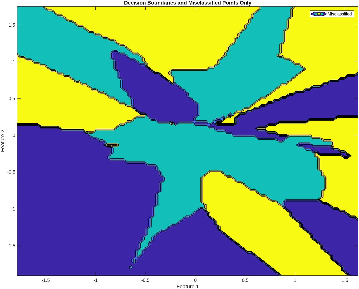
The following contains graphs of the training process:
P2
Implement in Matlab the bisection and Newton’s method for finding roots of scalar equations.
Use your implementation of the bisection method to find a root of
a. in
b. in .
Use your implementation of Newton’s method and Matlab’s fsolve to find a root of
a. with initial guess
b. with initial guess
For the bisection method, use . For your Newton and fsolve, solve until .
If you are obtaining different roots, explain the differences. Also, discuss the number of iterations.
Solution
Bisection method
function [root, fval, iter] = bisection(f, a, b, tol)
    if f(a) * f(b) >= 0
        error('f(a) and f(b) must have opposite signs');
    end

    iter = 0;
    while (b - a) / 2 > tol
        iter = iter + 1;
        c = (a + b) / 2;
        if f(c) == 0
            break;
        end
        if f(a) * f(c) < 0
            b = c;
        else
            a = c;
        end
    end
    root = (a + b) / 2;
    fval = f(root);
end

f1 = @(x) 1/x - exp(2 - sqrt(x));
a1 = 0.1; b1 = 1; tol = 1e-9;
[root_bisect1, fval_bisect1, iter_bisect1] = bisection(f1, a1, b1, tol);

f2 = @(x) x*sin(x) - 1;
a2 = 0; b2 = 2;
[root_bisect_2, fval_bisect_2, iter_bisect_2] = bisection(f2, a2, b2, tol);
Newton method
function [root, fval, iter] = newton(f, df, x0, tol)
    maxIter = 1000; % Limit number of iterations to prevent infinite loop
    iter = 0;
    x = x0;
    fx = f(x);

    while abs(fx) > tol && iter < maxIter
        iter = iter + 1;
        x = x - fx / df(x);
        fx = f(x);
    end

    root = x;
    fval = fx;
end

df1 = @(x) -1/x^2 + (1/(2*sqrt(x))) * exp(2 - sqrt(x));
x1 = 1;
[root_newton_1, fval_newton_1, iter_newton_1] = newton(f1, df1, x1, tol);

df2 = @(x) sin(x) + x*cos(x);
x2 = 2;
[root_newton_2, fval_newton_2, iter_newton_2] = newton(f2, df2, x2, tol);
fsolve
options = optimoptions('fsolve', 'Display', 'off', 'FunctionTolerance', 1e-9);
[root_fsolve_1, fval_fsolve_1, exitflag_1, output_1] = fsolve(f1, x1, options);
iter_fsolve_1 = output_1.iterations;

[root_fsolve_2, fval_fsolve_2, exitflag_2, output_2] = fsolve(f2, x2, options);
iter_fsolve_2 = output_2.iterations;
Table
For
| method | root | num. iterations | |
|---|---|---|---|
| bisection | 0.2152 | 8.7809e-09 | 29 |
| Newton | 28.6942 | -2.5223e-14 | 9 |
fsolve | 28.5131 | -3.7357e-04 | 12 |
For
| method | root | num. iterations | |
|---|---|---|---|
| bisection | 1.1142 | 4.3660e-10 | 30 |
| Newton | -9.3172 | -2.4834e-11 | 5 |
fsolve | 1.1142 | -1.9488e-08 | 3 |
Analysis
For
-
Bisection method: The bisection method found a root in the interval as expected. This method guarantees convergence to a root when it exists within the interval and the function changes sign. However, it is generally slower, as indicated by the higher number of iterations.
-
Newton’s method: converged to a completely different root, which is outside the interval considered for the bisection method. This shows that Newton’s method is highly sensitive to the initial guess. It also converges faster (fewer iterations) but can lead to roots that are far from the initial guess if the function is complex or if the derivative does not behave well.
-
fsolve: Similar to Newton’s method,fsolvealso found a root far from the interval used for the bisection method. Likely uses a variant of Newton’s method or a similar approach, which explains the similar behavior.
For
-
Bisection method: As with the first function, the bisection method finds a root within the specified interval. The method is reliable but slow, as seen from the number of iterations.
-
Newton’s method: converged to a negative root, which is quite far from the interval . This indicates that for this particular function, the method diverged significantly from the initial guess due to the function’s complex behavior, especially when considering trigonometric functions combined with polynomial terms.
Discussion:
-
Root Differences: The significant differences in roots, especially for Newton’s method and
fsolve, highlight the sensitivity of these methods to initial guesses and the nature of the function. For complex functions, especially those with multiple roots, the choice of the initial guess can lead to convergence to entirely different roots. -
Number of Iterations: Newton’s method and
fsolvegenerally require fewer iterations than the bisection method, demonstrating their faster convergence rate. However, this comes at the cost of potentially finding different roots, as seen in the results.
P3
The annuity equation is
where is borrowed amount, is the amount of each payment, is the interest rate per period, and there are equally spaced payments.
-
Write Newton’s method for finding .
-
Implement the function
function r = interest(A, n, P)which returns the annual interest rate. Your function must callfsolve. Ensure thatfsolveuses the analytical form of the derivative. Report the values ofinterest(100000, 20*12, 1000), interest(100000, 20*12, 100). Interpret the results.
Solution
Newton’s function for finding
Given
We have
Newton’s methods says , with
Thus,
Implementation
function r = interest(A, n, P)
    % Define the function f(r)
    function value = f(r)
        value = P/r * (1 - (1 + r)^-n) - A;
    end

    % Define the derivative f'(r)
    function value = df(r)
        value = -P/r^2 * (1 - (1 + r)^-n) + P*n/r * (1 + r)^(-n-1);
    end

    % Initial guess for r
    r_initial = 0.05; % A typical starting value for interest rates

    % Solve for r using fsolve
    options = optimoptions('fsolve', 'Display', 'none', 'SpecifyObjectiveGradient', true);
    r = fsolve(@(r) deal(f(r), df(r)), r_initial, options);
end

f_1000=interest(100000, 20*12, 1000)
f_100=interest(100000, 20*12, 100)
From calculation, f_100=-0.0099 and f_1000=0.0500. Given here that we use r_0=0.05 (or 5% interests rate)
For , the interest rate that satisfies the annuity equation is approximately 5%
For , the interest rate required to satisfy the loan conditions would have to be different from 5%. The negative value of the function (-0.0099) suggests that the actual interest rate required to meet the annuity equation under these conditions is lower than the initial guess of 5%.
Note that the initial value here affects Newton’s approximation vastly. If one changes to 1% one might observe different value
P4
Consider Newton’s method on
a. How do the computed approximations behave with ?
b. Try your implementation with and . Explain why this method behaves differently, when started with , compared to when it is started with .
c. Solve also with fsolve. Comment on the results.
Solution
Given the Newton’s implementation
function [root, fval, iter] = newton(f, df, x0, tol)
    maxIter = 1000; % Limit number of iterations to prevent infinite loop
    iter = 0;
    x = x0;
    fx = f(x);

    while abs(fx) > tol && iter < maxIter
        iter = iter + 1;
        x = x - fx / df(x);
        fx = f(x);
    end

    root = x;
    fval = fx;
end

% Define the function and its derivative
f = @(x) x.^5 - x.^3 - 4*x;
df = @(x) 5*x.^4 - 3*x.^2 - 4;

% Initial guess x0 = 1
x0 = 1;
tol = 1e-10;

root = newton(f, df, x0, tol);
disp(root);

% Initial guess x0 = 1 + 10^-14
x0 = 1 + 1e-14;
root = newton(f, df, x0, tol);
disp(root);
a. The approximation converges to . This indicates that the method finds a root at .
b. Newton’s Method with : The approximation converges to . This indicates that the method finds a root at .
Newton’s Method with : The approximation converges to a different value, approximately . This suggests that a small change in the initial guess leads Newton’s method to converge to a different root, highlighting the method’s sensitivity to initial conditions.
c. Using fsolve
options = optimoptions('fsolve','Display','none'); % Suppress fsolve output
root_fsolve = fsolve(f, 1, options);
disp(root_fsolve);
The fsolve result differs from the Newton’s method result for the same initial guess (yields 0). This could be due to the inherent differences in the algorithms used by fsolve.
fsolve in matlab uses Levenberg-Marquardt, which finds roots approximately by minimizing the sum of squares of the function and is quite robust, comparing to the heuristic implementation of the Newton’s implementation.
P5
Implement Newton’s method for systems of equations.
Each of the following systems of nonlinear equations may present some difficulty in computing a solution. Use Matlab’s fsolve and your own implementation of Newton’s method to solve each of the systems from the given starting point.
In some cases, the nonlinear solver may fail to converge or may converge to a point other than a solution. When this happens, try to explain the reason for the observed behavior.
Report for fsolve and your implementation of Newton’s method and each of the systems below, the number of iterations needed to achieve accuracy of (if achieved).


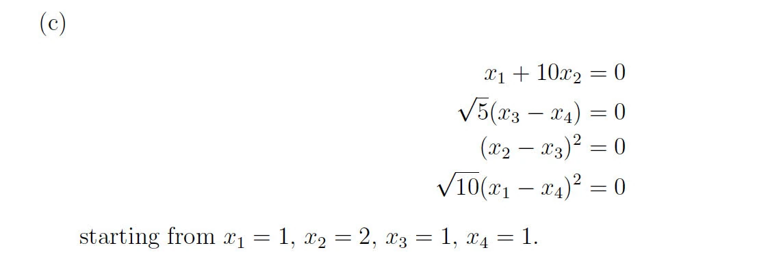

Solution
For all of the following Newton’s method implementation, it will follow the following framework
function p5
    % Define the system of equations F
    function F = equations(x) end

    % Define the Jacobian of the system
    function J = jacobian(x) end

    % Initial guess
    x0 = ...;

    % Tolerance and maximum number of iterations
    tol = 1e-6;
    max_iter = 100;

    % Newton's method
    x = x0;
    for iter = 1:max_iter
        F_val = equations(x);
        J_val = jacobian(x);
        delta = -J_val \ F_val; % Solve for the change using the backslash operator
        x = x + delta; % Update the solution

        % Check for convergence
        if norm(delta, Inf) < tol
            fprintf('Newton''s method: Solution found after %d iterations.\n', iter);
            fprintf('x1 = %.6f, x2 = %.6f\n', x(1), x(2));
            break;
        end
    end
    if iter == max_iter
        fprintf('Newton''s method: No solution found after %d iterations.\n', max_iter);
    end

    % fsolve method
    options = optimoptions('fsolve', 'Display', 'off', 'TolFun', tol, 'MaxIterations', max_iter);
    [x_fsolve, ~, exitflag, output] = fsolve(@equations, x0, options);

    if exitflag > 0 % fsolve converged to a solution
        fprintf('fsolve: Solution found after %d function evaluations.\n', output.funcCount);
        fprintf('x1 = %.6f, x2 = %.6f\n', x_fsolve(1), x_fsolve(2));
    else
        fprintf('fsolve: No solution found, exit flag = %d.\n', exitflag);
    end
end
Where equations is the Newton’s system of equations, jacobian is the Jacobian of the system, followed by x as the approximation and check for convergence.
A.
function p5
   % Define the system of equations
    function F = equations(x)
        F = zeros(2,1); % Ensure F is a column vector
        F(1) = x(1) + x(2)*(x(2)*(5 - x(2)) - 2) - 13;
        F(2) = x(1) + x(2)*(x(2)*(1 + x(2)) - 14) - 29;
    end

    % Define the Jacobian of the system
    function J = jacobian(x)
        J = zeros(2,2); % Initialize J as a 2x2 matrix
        J(1,1) = 1;
        J(1,2) = (5 - 3*x(2))*x(2) - 2;
        J(2,1) = 1;
        J(2,2) = (1 + 3*x(2))*x(2) - 14;
    end

    % Initial guess
    x0 = [15; -2];

    % Tolerance and maximum number of iterations
    tol = 1e-6;
    max_iter = 100;

    % Newton's method
    x = x0;
    for iter = 1:max_iter
        F_val = equations(x);
        J_val = jacobian(x);
        delta = -J_val \ F_val; % Solve for the change using the backslash operator
        x = x + delta; % Update the solution

        % Check for convergence
        if norm(delta, Inf) < tol
            fprintf('Newton''s method: Solution found after %d iterations.\n', iter);
            fprintf('x1 = %.6f, x2 = %.6f\n', x(1), x(2));
            break;
        end
    end
    if iter == max_iter
        fprintf('Newton''s method: No solution found after %d iterations.\n', max_iter);
    end

    % fsolve method
    options = optimoptions('fsolve', 'Display', 'off', 'TolFun', tol, 'MaxIterations', max_iter);
    [x_fsolve, ~, exitflag, output] = fsolve(@equations, x0, options);

    if exitflag > 0 % fsolve converged to a solution
        fprintf('fsolve: Solution found after %d function evaluations.\n', output.iterations);
        fprintf('x1 = %.6f, x2 = %.6f\n', x_fsolve(1), x_fsolve(2));
    else
        fprintf('fsolve: No solution found, exit flag = %d.\n', exitflag);
    end
end
yields
Newton's method: Solution found after 23 iterations.
x1 = 5.000000, x2 = 4.000000
fsolve: No solution found, exit flag = -2.
Since Newton’s method is locally convergent, meaning that if the starting point is close enough to the actual solution, it will usually converge quickly, and in this case, it did. This means the initial guess was sufficiently close with the true solution.
However, fsolve did not converge to a solution. Since fsolve uses Levenberg-Marquardt algorithm (This algorithm is a trust-region type algorithm![]() , which is a combination of the Gauss-Newton algorithm and the method of gradient descent), it does come with limitation:
, which is a combination of the Gauss-Newton algorithm and the method of gradient descent), it does come with limitation:
- The Levenberg-Marquardt algorithm can be sensitive to the starting values. If the initial guess is not sufficiently close to the true solution, the algorithm may not converge. (which we observed)
- Local minima: The algorithm may converge to a local minimum instead of a global minimum, especially if the function landscape is complex with multiple minima.
exit flag of -2 means that the two consecutive steps taken by the algorithm were unable to decrease the residual norm, and the algorithm terminated prematurely.
B
function p5
   % Define the system of equations
    function F = equations(x)
        F = zeros(3,1); % Ensure F is a column vector
        F(1) = x(1)^2 + x(2)^2 + x(3)^2 - 5;
        F(2) = x(1) + x(2) - 1;
        F(3) = x(1) + x(3) - 3;
    end

    % Define the Jacobian of the system
    function J = jacobian(x)
        J = zeros(3,3); % Initialize J as a 3x3 matrix
        J(1,1) = 2*x(1);
        J(1,2) = 2*x(2);
        J(1,3) = 2*x(3);
        J(2,1) = 1;
        J(2,2) = 1;
        J(2,3) = 0;
        J(3,1) = 1;
        J(3,2) = 0;
        J(3,3) = 1;
    end

    % Initial guess
    x0 = [(1+sqrt(3))/2; (1-sqrt(3))/2; sqrt(3)];

    % Tolerance and maximum number of iterations
    tol = 1e-6;
    max_iter = 100;

    % Newton's method
    x = x0;
    for iter = 1:max_iter
        F_val = equations(x);
        J_val = jacobian(x);
        delta = -J_val \ F_val; % Solve for the change using the backslash operator
        x = x + delta; % Update the solution

        % Check for convergence
        if norm(delta, Inf) < tol
            fprintf('Newton''s method: Solution found after %d iterations.\n', iter);
            fprintf('x1 = %.6f, x2 = %.6f, x3 = %.6f\n', x(1), x(2), x(3));
            break;
        end
    end
    if iter == max_iter
        fprintf('Newton''s method: No solution found after %d iterations.\n', max_iter);
    end

    % fsolve method
    options = optimoptions('fsolve', 'Display', 'off', 'TolFun', tol, 'MaxIterations', max_iter);
    [x_fsolve, ~, exitflag, output] = fsolve(@equations, x0, options);

    if exitflag > 0 % fsolve converged to a solution
        fprintf('fsolve: Solution found after %d function evaluations.\n', output.iterations);
        fprintf('x1 = %.6f, x2 = %.6f, x3 = %.6f\n', x_fsolve(1), x_fsolve(2), x_fsolve(3));
    else
        fprintf('fsolve: No solution found, exit flag = %d.\n', exitflag);
    end
end
yields
Newton's method: Solution found after 57 iterations.
x1 = 1.666667, x2 = -0.666667, x3 = 1.333333
fsolve: Solution found after 6 function evaluations.
x1 = 1.000000, x2 = 0.000000, x3 = 2.000000
Newton’s method takes steps based directly on the local derivative information, potentially taking large steps when far from the solution and smaller steps when closer. fsolve, when using the Levenberg-Marquardt algorithm, combines aspects of the gradient descent method (which takes smaller, more cautious steps) with the Gauss-Newton method (which is more aggressive). This can lead to different paths through the solution space and convergence to different solutions
fsolve might have found a local minimum, which it mistook for a global minimum, while Newton’s method might have bypassed this due to its larger initial steps.
C
function p5
   % Define the system of equations
    function F = equations(x)
        F = zeros(4,1); % Ensure F is a column vector
        F(1) = x(1) + x(2)*10;
        F(2) = sqrt(5)*(x(3) - x(4));
        F(3) = (x(2)-x(3))^2;
        F(4) = sqrt(10)*(x(1)-x(4))^2;
    end

    % Define the Jacobian of the system
    function J = jacobian(x)
        J = zeros(4,4); % Initialize J as a 3x3 matrix
        J(1, :) = [1, 10, 0, 0];
        J(2, :) = [0, 0, sqrt(5), -sqrt(5)];
        J(3, :) = [0, 2*(x(2) - x(3)), -2*(x(2) - x(3)), 0];
        J(4, :) = [2*sqrt(10)*(x(1) - x(4)), 0, 0, -2*sqrt(10)*(x(1) - x(4))];
    end

    % Initial guess
    x0 = [1; 2; 1; 1];

    % Tolerance and maximum number of iterations
    tol = 1e-6;
    max_iter = 100;

    % Newton's method
    x = x0;
    for iter = 1:max_iter
        F_val = equations(x);
        J_val = jacobian(x);
        delta = -J_val \ F_val; % Solve for the change using the backslash operator
        x = x + delta; % Update the solution

        % Check for convergence
        if norm(delta, Inf) < tol
            fprintf('Newton''s method: Solution found after %d iterations.\n', iter);
            fprintf('x1 = %.6f, x2 = %.6f, x3 = %.6f, x4 = %.6f\n', x);
            break;
        end
    end
    if iter == max_iter
        fprintf('Newton''s method: No solution found after %d iterations.\n', max_iter);
    end

    % fsolve method
    options = optimoptions('fsolve', 'Display', 'iter', 'TolFun', tol, 'MaxIterations', max_iter);
    [x_fsolve, fval, exitflag, output] = fsolve(@equations, x0, options);

    if exitflag > 0 % fsolve converged to a solution
        fprintf('fsolve: Solution found after %d function evaluations.\n', output.funcCount);
        fprintf('x1 = %.6f, x2 = %.6f, x3 = %.6f, x4 = %.6f\n', x_fsolve);
    else
        fprintf('fsolve: No solution found, exit flag = %d.\n', exitflag);
    end
end
yields
Newton's method: No solution found after 100 iterations.
fsolve: Solution found after 35 function evaluations.
x1 = -0.002673, x2 = 0.000267, x3 = 0.000407, x4 = 0.000407
Newton’s method cannot find convergence after 100 steps because of divergence, if the initial guess is not close to the root, especially in the presence of steep gradients or saddle points. The Jacobian matrix at some point during the iteration may become ill-conditioned, which would lead to large numerical errors in the computation of the inverse or the solution of the linear system in each iteration
fsolve converged here, meaning Levenberg-Marquardt is probably more robust in converging a local minima in this case.
D
function p5
   % Define the system of equations
    function F = equations(x)
        F = zeros(2,1); % Ensure F is a column vector
        F(1) = x(1);
        F(2) = 10*x(1) / (x(1) + 0.1) + 2*x(2)^2;
    end

    % Define the Jacobian of the system
    function J = jacobian(x)
        J = zeros(2,2); % Initialize J as a 2x2 matrix
        J(1, :) = [1, 0];
        J(2, :) = [10*(0.1)/(x(1) + 0.1)^2, 4*x(2)];
    end

    % Initial guess
    x0 = [1.8; 0];

    % Tolerance and maximum number of iterations
    tol = 1e-6;
    max_iter = 100;

    % Newton's method
    x = x0;
    for iter = 1:max_iter
        F_val = equations(x);
        J_val = jacobian(x);
        delta = -J_val \ F_val; % Solve for the change using the backslash operator
        x = x + delta; % Update the solution

        % Check for convergence
        if norm(delta, Inf) < tol
            fprintf('Newton''s method: Solution found after %d iterations.\n', iter);
            fprintf('x1 = %.6f, x2 = %.6f\n', x(1), x(2));
            break;
        end
    end
    if iter == max_iter
        fprintf('Newton''s method: No solution found after %d iterations.\n', max_iter);
    end

    % fsolve method
    options = optimoptions('fsolve', 'Display', 'off', 'TolFun', tol, 'MaxIterations', max_iter);
    [x_fsolve, ~, exitflag, output] = fsolve(@equations, x0, options);

    if exitflag > 0 % fsolve converged to a solution
        fprintf('fsolve: Solution found after %d function evaluations.\n', output.iterations);
        fprintf('x1 = %.6f, x2 = %.6f\n', x_fsolve(1), x_fsolve(2));
    else
        fprintf('fsolve: No solution found, exit flag = %d.\n', exitflag);
    end
end
yields
Newton's method: No solution found after 100 iterations.
fsolve: Solution found after 15 function evaluations.
x1 = 0.000000, x2 = -0.000316
For Newton’s method:
- Non-convergence: The fact that Newton’s method did not converge could be due to several factors such as a poor initial guess, especially since is one of the solutions, which may lead to a division by zero or a derivative that does not exist at some point during the iteration.
- Sensitive Derivative: The function has a derivative that becomes very large as approaches -0.1, and this can cause numerical issues, such as overflow or large rounding errors, which can prevent convergence.
- Flat Regions: The method might be getting stuck in a flat region of the function where the gradient is very small, leading to very small steps that do not significantly change the estimate of the solution.
For fsolve observation, same arguments can be made that of similar to problem C observation, with regards to robustness of Levenberg-Marquardt algorithm in solving this system of non-linear equations.
P6
You are given the data file data.txt. Each row contains the 2D
coordinates of an object at time . This object exhibits a periodic motion.
Implement the function function period = findPeriod(file_name)
that reads the data from a file and computes the period of the periodic motion.
The points in time where the object returns to the same position must be determined using fsolve. Report the value for the computed period.
Solution
function period = findPeriod(file_name)
    % Parse the data from the file
    data = parse(file_name);

    % Extract time, x, and y coordinates
    t = data(:, 1);
    x = data(:, 2);
    y = data(:, 3);

    % Define a tolerance for how close the object needs to be to its initial position
    tolerance = 1e-9;

    % Define interpolation functions for x and y, restricted to the range of data
    x_interp = @(tq) interp1(t, x, tq, 'spline', 'extrap');
    y_interp = @(tq) interp1(t, y, tq, 'spline', 'extrap');

    % Define the distance function from the initial position
    distance_from_initial = @(tq) sqrt((x_interp(tq) - x(1))^2 + (y_interp(tq) - y(1))^2);

    % Initial guess for fsolve - use the midpoint of the time data
    initial_guess = t(floor(length(t)/2));

    % Use fsolve to find the time at which the distance is minimized
    options = optimoptions('fsolve', 'Display', 'iter', 'TolFun', tolerance, 'MaxFunEvals', 10000);
    t_period = fsolve(distance_from_initial, initial_guess, options);

    % Calculate the period
    period = t_period - t(1);
end

function data = parse(file_name)
    % Open the file
    fid = fopen(file_name, 'rt');
    if fid == -1
        error('Failed to open file: %s', file_name);
    end

    % Read the data from the file
    % Assuming the data is separated by spaces or tabs
    data = fscanf(fid, '%f %f %f', [3, Inf]);

    % Transpose the data to have rows as individual entries
    data = data';

    % Close the file
    fclose(fid);
end
yields the computed period of 39.3870
P7
Consider two bodies of masses and (Earth and Sun) in a planar motion, and a third body of negligible mass (moon) moving in the same plane. The motion is given by
and
The initial values are , , , .
Implement the classical Runge-Kutta method of order 4 and integrate this problem on with uniform stepsize using 100, 1000, 10,000, and 20,000 steps.
Plot the orbits for each case. How many uniform steps are needed before the orbit appears to be qualitatively correct?
Submit plots and discussion.
Solution
function rk4
    % Constants
    mu = 0.012277471;
    mu_hat = 1 - mu;

    % Initial Conditions
    u0 = [0.994, 0, 0, -2.001585106379082522420537862224];

    % Time Span
    t_span = [0 17.1];

    % Solve for different step sizes
    step_sizes = [100, 1000, 10000, 20000];
    for i = 1:length(step_sizes)
        solve_with_steps(t_span, u0, step_sizes(i), mu, mu_hat);
    end
end

function solve_with_steps(t_span, u0, steps, mu, mu_hat)
    % RK4 Integration
    h = (t_span(2) - t_span(1)) / steps;
    t = linspace(t_span(1), t_span(2), steps);
    u = zeros(length(u0), length(t));
    u(:,1) = u0';

    for i = 1:length(t)-1
        k1 = equations(t(i), u(:,i), mu, mu_hat);
        k2 = equations(t(i) + h/2, u(:,i) + h/2*k1, mu, mu_hat);
        k3 = equations(t(i) + h/2, u(:,i) + h/2*k2, mu, mu_hat);
        k4 = equations(t(i) + h, u(:,i) + h*k3, mu, mu_hat);

        u(:,i+1) = u(:,i) + h/6 * (k1 + 2*k2 + 2*k3 + k4);
    end

    % Plotting
    figure;
    plot(u(1,:), u(3,:));
    xlabel('u1');
    ylabel('u2');
    title(sprintf('Orbit of the Third Body with RK4 (%d Steps)', steps));
    grid on;

    % NOTE: The below is the correct approximation using ode45,
    % but for the sake of this assignment, we implement RK4
    % t_eval = linspace(t_span(1), t_span(2), steps);
    % [T, U] = ode45(@(t,u) equations(t, u, mu, mu_hat), t_eval, u0);
    % % Plotting
    % figure;
    % plot(U(:,1), U(:,3));
    % xlabel('u1');
    % ylabel('u2');
    % title(sprintf('Orbit of the Third Body (%d Steps)', steps));
    % grid on;
end

function dudt = equations(t, u, mu, mu_hat)
    u1 = u(1);
    u1_prime = u(2);
    u2 = u(3);
    u2_prime = u(4);

    delta1 = ((u1 + mu)^2 + u2^2)^1.5;
    delta2 = ((u1 - mu_hat)^2 + u2^2)^1.5;

    du1dt = u1_prime;
    du1_primedt = u1 + 2*u2_prime - mu_hat*(u1 + mu)/delta1 - mu*(u1 - mu_hat)/delta2;
    du2dt = u2_prime;
    du2_primedt = u2 - 2*u1_prime - mu_hat*u2/delta1 - mu*u2/delta2;

    dudt = [du1dt; du1_primedt; du2dt; du2_primedt];
end
yields the following graph
100 steps
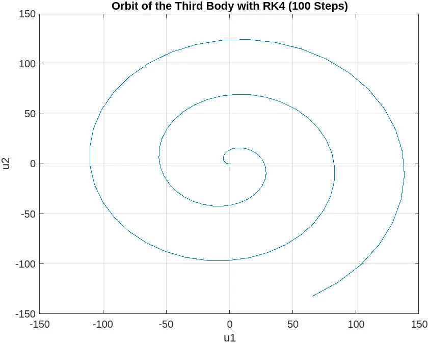
It appears that the plot for the first 100 steps of the three-body problem using the RK4 method in MATLAB shows a spiral pattern rather than the expected closed orbit. This divergence could be due to several factors:
Step Size: A step size of 100 may be too large to accurately capture the dynamics of the system, leading to significant numerical errors. The three-body problem is known for its sensitivity to initial conditions and step sizes, and thus requires a smaller step size for a more accurate solution.
Numerical Stability: The RK4 method, while fourth-order accurate for each step, is not guaranteed to be stable for all step sizes and problems.
1000 steps
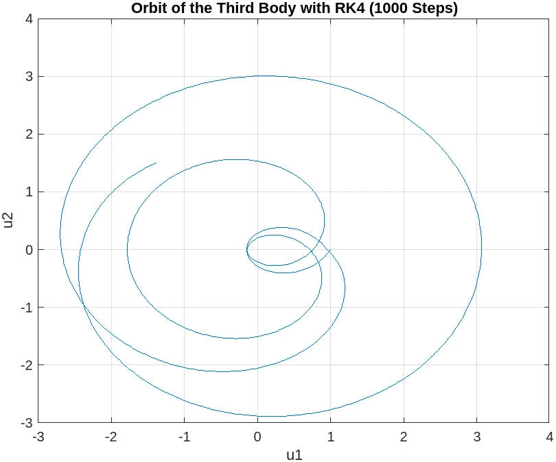
The plot for the 1000 steps case shows a significant improvement over the 100 steps case. This plot demonstrates a more defined and coherent orbit, which suggests that the step size is more appropriate for capturing the dynamics of the system. The spiral pattern from the 100 steps case is less pronounced, and the orbit begins to resemble the expected closed path of the three-body problem.
However, there is still some noticeable deviation and distortion in the orbit, which indicates that while the solution is converging towards the correct behavior with a smaller step size, further refinement might be necessary. In practice, continuing to reduce the step size can help further improve the accuracy of the orbit.
10000 steps
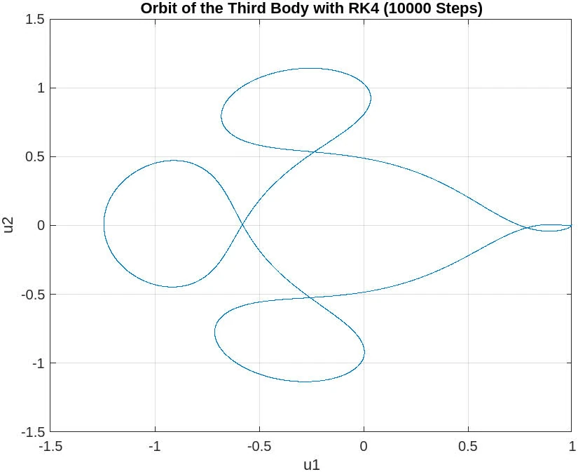
The plot for 10,000 steps demonstrates a substantial improvement and now depicts a closed orbit, which is characteristic of the three-body problem when solved with sufficient numerical accuracy. This indicates that a step size small enough to capture the system’s dynamics accurately has been achieved, and the RK4 method is yielding a reliable approximation of the moon’s orbit.
The orbit is smooth and does not exhibit the distortions seen in the plots with fewer steps. This suggests that the numerical integration is now sufficiently resolving the trajectory over the time span of interest. With 10,000 steps, it appears that the orbit is qualitatively correct, showing the expected behavior of a third body under the gravitational influence of the other two massive bodies.
Sufficient Resolution: The step size of 10,000 steps seems to provide a high enough resolution for the RK4 method to produce a stable and accurate orbit. Numerical Accuracy: The smaller step size has reduced the numerical errors to a level where they do not significantly affect the qualitative behavior of the solution. Orbit Stability: The closed and stable orbit indicates that the solution is likely converging to the true physical behavior of the system.
20000 steps
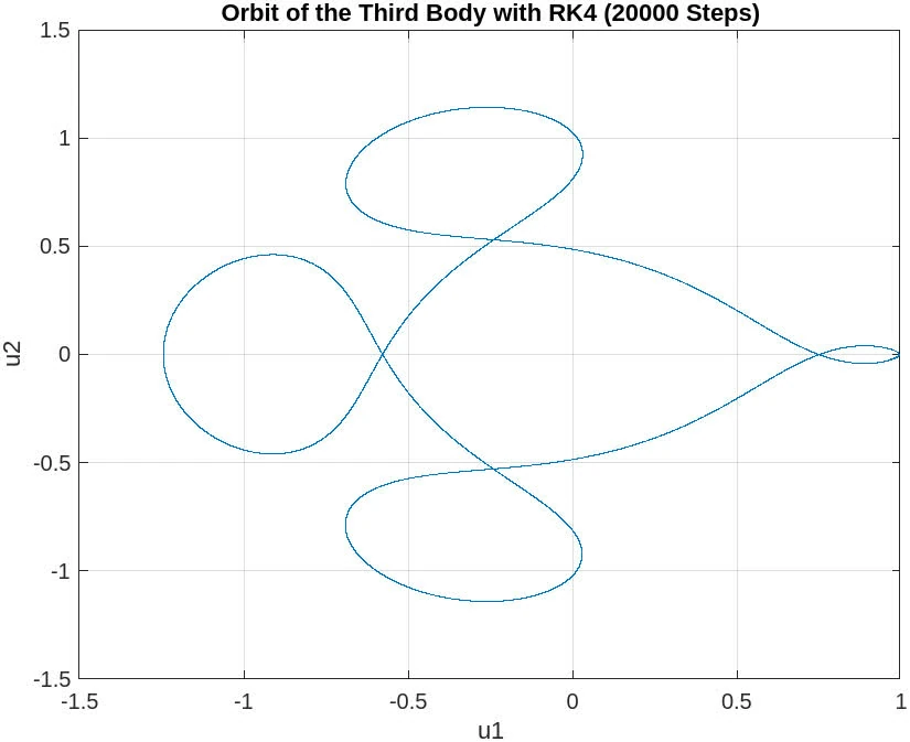
The plot for 20,000 steps exhibits a very stable and well-defined orbit, which closely resembles the plot for 10,000 steps. This consistency between the two resolutions suggests that the numerical solution has converged, and increasing the step count further does not result in any significant changes to the orbit’s shape or accuracy.
NOTE: The above implementation manually implement RK4, since ode45 is an adaptive methods and not conform to the fixed-step RK4. The equivalent of Python’s implementation with RK45.
P8
The following system of ODEs, formulated by Lorenz, represents are crude model of atmospheric circulation:
Set , take initial values , and integrate this ODE from using Matlab’s ode45.
Plot each component of the solution as a function of . Plot also , , and (in separate plots).
Change the initial values by a tiny amount (e.g. ) and integrate again. Compare the difference in the computed solutions.
Solution
function lorenz
    % Parameters
    sigma = 10;
    b = 8/3;
    r = 28;

    % Initial conditions
    y0 = [15; 15; 36];

    % Time span
    tspan = [0 100];

    % Solve the ODE
    [t, Y] = ode45(@(t,y) lorenzODE(t, y, sigma, b, r), tspan, y0);

    % Plotting the solutions
    figure;
    subplot(2, 2, 1);
    plot(t, Y(:,1), t, Y(:,2), t, Y(:,3));
    title('Time Series of y1, y2, y3');
    legend('y1', 'y2', 'y3');
    xlabel('Time');
    ylabel('Values');

    subplot(2, 2, 2);
    plot(Y(:,1), Y(:,2));
    title('y1 vs y2');
    xlabel('y1');
    ylabel('y2');

    subplot(2, 2, 3);
    plot(Y(:,1), Y(:,3));
    title('y1 vs y3');
    xlabel('y1');
    ylabel('y3');

    subplot(2, 2, 4);
    plot(Y(:,2), Y(:,3));
    title('y2 vs y3');
    xlabel('y2');
    ylabel('y3');

    % Modify initial conditions and solve again
    y0_mod = y0 + 1e-10;
    [t_mod, Y_mod] = ode45(@(t,y) lorenzODE(t, y, sigma, b, r), tspan, y0_mod);

    % Interpolate Y_mod to match the time points of t
    Y_mod_interp = interp1(t_mod, Y_mod, t);

    % Compute the differences
    Y_diff = Y - Y_mod_interp;

    % Plot the differences
    figure;
    plot(t, Y_diff);
    title('Difference in Solutions with Modified Initial Conditions');
    legend('Δy1', 'Δy2', 'Δy3');
    xlabel('Time');
    ylabel('Difference in Values');
end

function dydt = lorenzODE(t, y, sigma, b, r)
    % Lorenz system ODEs
    dydt = [sigma*(y(2) - y(1)); r*y(1) - y(2) - y(1)*y(3); y(1)*y(2) - b*y(3)];
end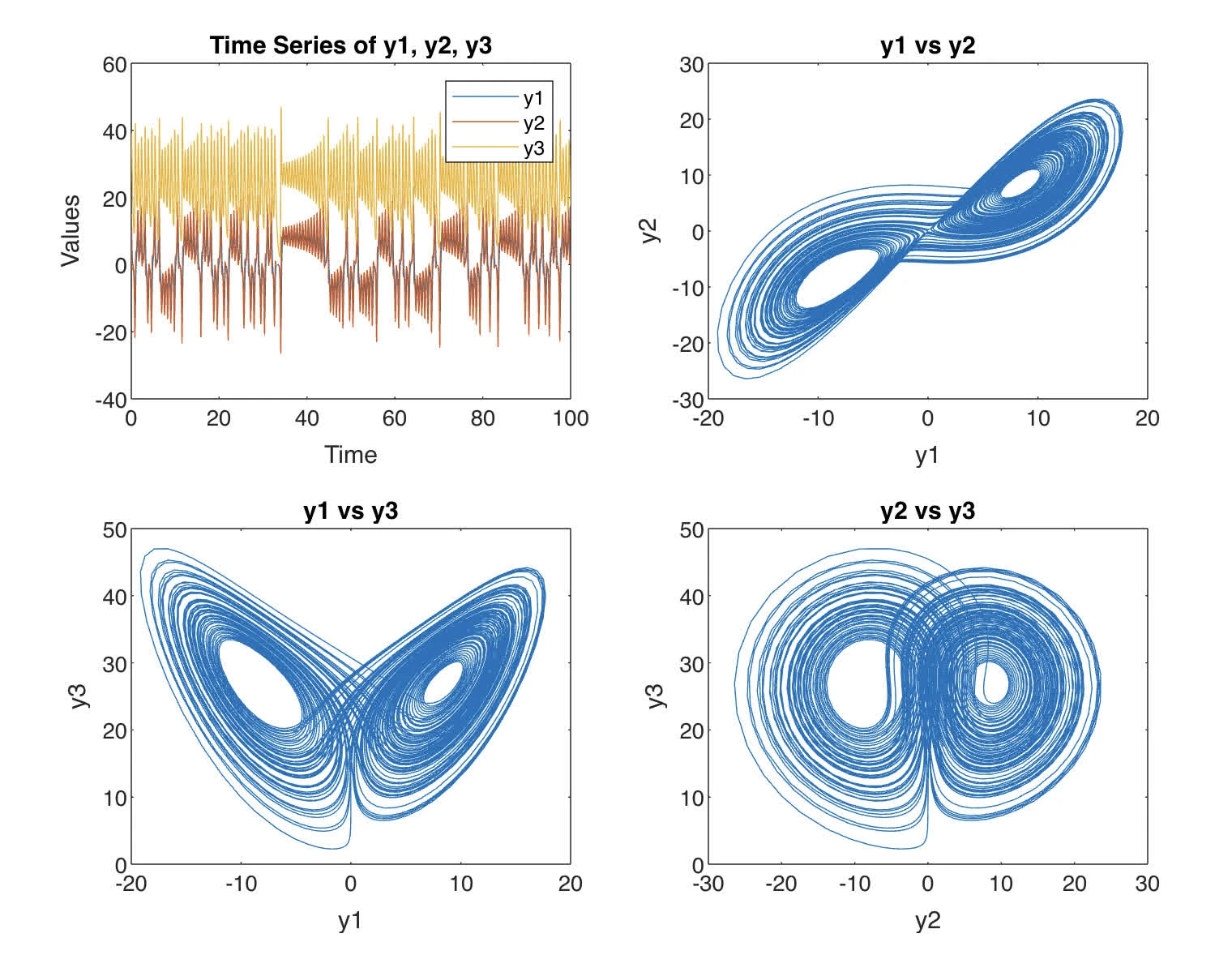
The difference between the time series graph as shown
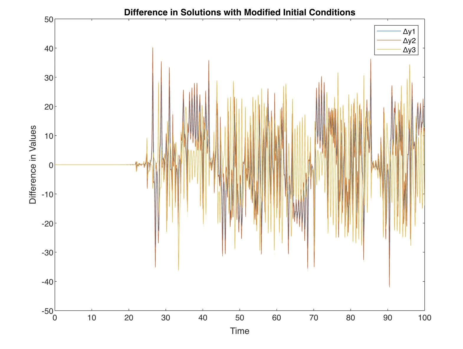 and diff between Lorenz are shown
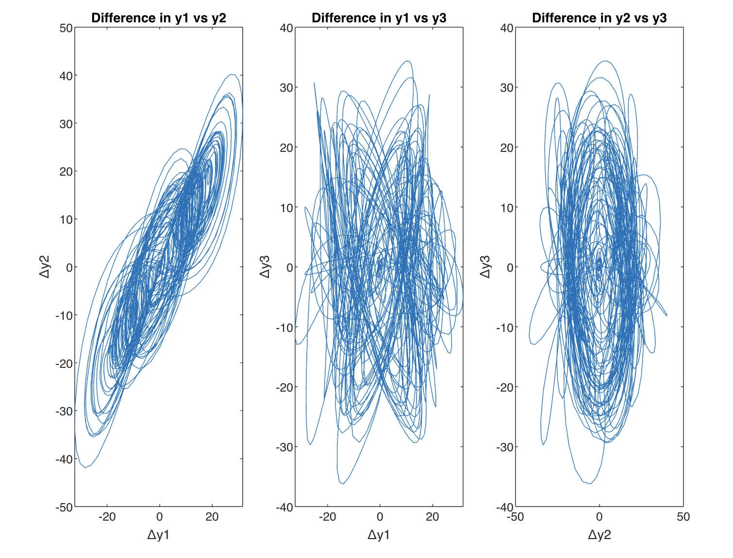
The difference in the time series of indicates how sensitive the Lorenz system is to initial conditions. Even though the change in the initial conditions is extremely small (on the order of ), the differences in the variables grow over time. This divergence is a characteristic of chaotic systems and is known as sensitivity to initial conditions or the butterfly effect.
Difference in Phase Space Graphs, or the delta plots show that the discrepancies between the two sets of solutions with slightly different initial conditions also exhibit complex behavior. Initially, the differences are small, but as time progresses, they become more pronounced, indicating that the system’s trajectory has deviated significantly from the original path.
P9
Let A be an singular matrix. Let
where is the identity matrix. When is the zero matrix, then .
We can use Newton’s method to find :
We replace by to obtain the formula (1)
a. Write a function to compute the inverse of a given matrix A using (1). You can use as an initial guess
Test your program on a few random matrices and report numerical experiments comparing its accuracy and efficiency with Matlab’s inverse function inv.
b. Does (1) converge quadratically? Provide sufficient detail supporting your claim.
Solution
a. The following entails the MATLAB solution (Python equivalent is inverse_newt.py)
function A_inv = matrix_inverse_newt(A)
    tol = 1e-9;
    max_iter = 100;
    n = size(A, 1);
    I = eye(n);
    Xk = A' / (norm(A, 1) * norm(A, inf));

    for k = 1:max_iter
        Rk = I - A * Xk;
        Xk_new = Xk + Xk * Rk;

        % Stopping criterion based on the norm of the residual matrix
        if norm(Rk) < tol
            break;
        end

        Xk = Xk_new;
    end

    A_inv = Xk;
end

% Test the function with a random matrix
rng(0); % Seed for reproducibility
n = 4; % Size of the matrix
A = rand(n, n);
A_inv = matrix_inverse_newt(A);

% Compare with MATLAB's built-in inverse function
A_inv_true = inv(A);

disp('Inverse using Newton''s method:');
disp(A_inv);
disp('True Inverse:');
disp(A_inv_true);
disp('Difference:');
disp(A_inv - A_inv_true);
yields
Inverse using Newton's method:
  -15.2997    3.0761   14.7235    9.6445
   -0.2088   -1.8442    1.0366    1.8711
   14.5694   -1.9337  -14.6497   -9.0413
   -0.3690    0.5345    1.4378   -0.4008

True Inverse:
  -15.2997    3.0761   14.7235    9.6445
   -0.2088   -1.8442    1.0366    1.8711
   14.5694   -1.9337  -14.6497   -9.0413
   -0.3690    0.5345    1.4378   -0.4008

Difference:
   1.0e-09 *

    0.6111   -0.1011   -0.6027   -0.3839
    0.0353   -0.0058   -0.0348   -0.0222
   -0.5881    0.0973    0.5800    0.3694
    0.0273   -0.0045   -0.0269   -0.0171
b. For quadratic convergence, we need
In this case, we need to check as k increases.
Substitute we have
Therefore, for quadratic convergence, we need for some constant
From this, we have
The following modification of Python implementation is used to track errors
import os, numpy as np

def errors(A):
  A_inv = matrix_inverse_newt(A)
# Recalculate the inverse and get the error at each iteration
  A_inv_newton, errors_newton = matrix_inverse_newt_err(A)
# Now we will check for quadratic convergence by calculating the ratio of errors
  ratios = []
  for i in range(1, len(errors_newton)-1):
      ratios.append(errors_newton[i+1] / errors_newton[i]**2)
  return ratios

def matrix_inverse_newt_err(A, tol=1e-9, max_iter=100):
    n = A.shape[0]
    I = np.eye(n)
    A_inv_true = np.linalg.inv(A) # True inverse for error calculation
    Xk = A.T / (np.linalg.norm(A, 1) * np.linalg.norm(A, np.inf))
    errors = [] # List to track errors over iterations
    for _ in range(max_iter):
        Rk = I - np.dot(A, Xk)
        Xk_new = Xk + np.dot(Xk, Rk)
        # Calculate and store the current error
        current_error = np.linalg.norm(Xk_new - A_inv_true)
        errors.append(current_error)
        # Stopping criterion based on the norm of the residual matrix
        if current_error < tol: break
        Xk = Xk_new
    return Xk, errors


if __name__ == "__main__":
  # Test the function with a random matrix
  np.random.seed(420)  # Seed for reproducibility
  n = 4  # Size of the matrix
  A = np.random.rand(n, n)
  print(errors(A))
From the Python implementation, we calculated the ratio of the error at step to the square of the error at step , and observed that these ratios seemed to stabilize around a constant value, rather than decreasing to zero. However, the ratios did not significantly deviate, indicating a consistent rate of convergence that could be quadratic.
To assert that the convergence is quadratic, we would expect the ratios to be bounded and for to be significantly less than as increases. The results from Python showed that the error does decrease from one iteration to the next, which is consistent with convergence.
The discrepancy between the theoretical expectation of quadratic convergence and the observed stabilisation of the error ratios might suggest that while the Newton’s method for matrix inversion is converging, it may not exhibit pure quadratic convergence in the empirical test we conducted. There could be several reasons for this: - The matrix used in the test may not meet the conditions required for quadratic convergence throughout the iterations. - The numerical precision and floating-point representation in Python may affect the calculation of the error and its ratios.