A multi-layer perceptron (MLP) architecture built on top of a multi-head attention mechanism (Vaswani et al., 2023) to signal high entropy tokens to be amplified and less important tokens to be diminished.
ELI5: Mom often creates a food list consists of n of items to buy. Your job is to guess what the last item on this list would be.
Most implementations are autoregressive. Most major SOTA are decoder-only, as encoder-decoder models has lack behind due to their expensive encoding phase.
llama.cpp surprised many people (myself included) with how quickly you can run large LLMs on small computers, e.g. 7B runs @ ~16 tok/s on a MacBook. Wait don't you need supercomputers to work… pic.twitter.com/EIp9iPkZ6x
EAGLE-1’s limitation at its feature prediction constraints, via LM head architecture,
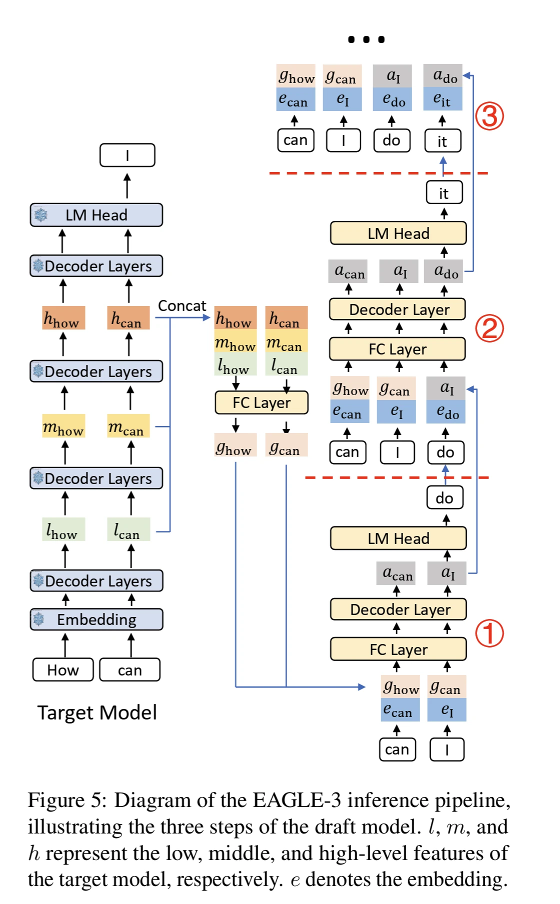
EAGLE-3 addresses this by use direct token prediction and rely on multi-layer feature fusion called “training-time test”, similar to MLP Speculator
distribution skew
EAGLE does not involve any fine-tuning of the target model, therefore preservation of outputs distributions by EAGLE is theoretically guaranteed for both greedy and non-greedy sampling. This is not the case with Lookahead and Medusa.
EAGLE-1
Observations:
autoregressive on feature-level 1 is simpler than token-level, given that there are more regularity.
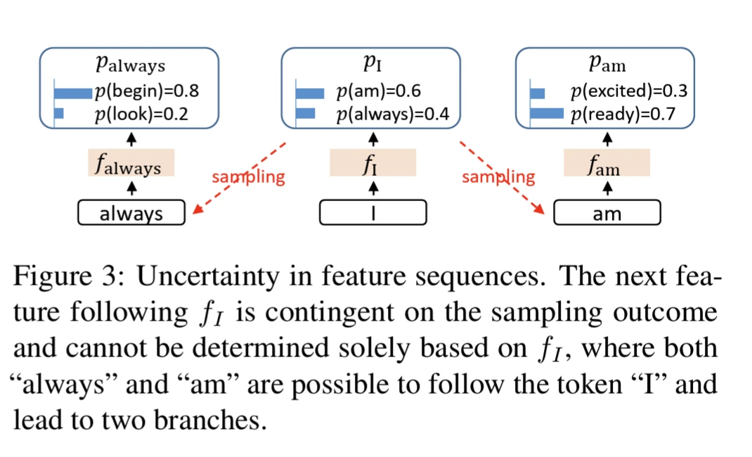
uncertainty in sampling process hinders the performance of predicting the next feature.
feature-level are high-dimensional and continuous, meaning sampling “am” or “always” will results in different feature sequences.
EAGLE address this by inputs the token sequence from one time step ahead including the sampling outcomes into the draft models.
predicting falways based on fI and talways
predicting fam based on fI and tam
notation.
“Features” refers to second-to-top-layer feature of LLM, or the hidden states before LM head
Token by t, embedding by e, features by f, distributions by p
Sequences are referred as Ti:j for (ti,ti+1,…,tj)2
idea: to use string matching from prompt to generate candidate tokens, instead of using a draft-based models.
def find_candidate_pred_tokens(input_ids, max_ngram_size=3, num_pred_tokens=10):
  input_length = input_ids.size(1)

  for ngram_size in range(max_ngram_size, 0, -1):
    # Extract the last n tokens as our search ngram
    ngram = input_ids[0, -ngram_size:].tolist()

    # Create sliding windows of size ngram_size
    windows = input_ids.unfold(dimension=1, size=ngram_size, step=1)

    # Convert ngram to a tensor for comparison
    ngram_tensor = torch.tensor(ngram, device=input_ids.device).unsqueeze(0)

    # Find where the windows match the ngram
    matches = (windows == ngram_tensor).all(dim=2)

    # Get the indices of matches
    match_indices = matches.nonzero(as_tuple=True)[1]

    # Iterate through match indices to find a valid continuation
    for idx in match_indices:
      start_idx = idx + ngram_size
      end_idx = start_idx + num_pred_tokens
      # Ensure we don't go beyond the length of input_ids and avoid self-match
      if end_idx <= input_length and start_idx < input_length - ngram_size:
        return input_ids[0, start_idx:end_idx]

  # If no match is found, return an empty tensor
  return torch.tensor([], dtype=torch.long, device=input_ids.device)
Latency is improved at the cost of increasing ops, meaning 2x-3x with T5, with a scale of γ=5 (also referred in practice as num_speculative_tokens)
This is not useful when computation resources are limited.
Walltime improvement by (1−α)(γc+1)1−αγ+1 where α is the approximation E(β) (or natural measure of the acceptance rate β)
Note that this is different from rejection sampling 6, given that non-iterative rejection sampling would yield lower acceptance rate
Lenience factor l to perform speed versus quality trade-off 7 when draft-models distributions is different from target-models’. Note that we can’t use temperature=0 (i.e argmax sampling).
Instead we allow some lenience before standardizing the distribution (accept token x sampled from Mq in case of p(x)≤lmax˙p)
In this case, then similar empirical increases to α to those of temperature=1
goal and algorithm
Let Mp be the target model for task X, and p(xt∣x<t) the distribution we get from model for a prefix x<t
Let Mq be the draft/approximation models at the same task, and q(xt∣x<t) the distribution we get from model for a prefix x<t
Objective: to use Mq to generate γ∈Z+ completions, and use Mp to verify γ tokens in parallel
Keep when q(x)≤p(x)
Reject when q(x)≥p(x) for sample with P=1−q(x)p(x) and sample x again from p′(x)=norm(max(0,p(x)−q(x)))8
With i.i.d assumption speculative sampling reduces # of calls to target models by 1−α1−αγ+1, assuming running on compute resources that support increased concurrency (GPUs.)
For walltime 11 analysis, assuming we can run γ+1 concurrent evaluation of Mp:
cost-efficient
let c be the ratio between time for single run of Mq and the time for single run Mp
c is highly dependent on hardware measure. From the paper, c≈0 to avoid expectancy biases
Theorem 3.8
expected improvement factor in total walltime by (1−α)(γc+1)1−αγ+112
Note that we assume there are long enough generations sequence here.
Corollary 3.9
∀α>c∃γ∣ we will get improvement by a factor of 1+c1+α
If we get an improvement for γ, we’d also get improvement for any 0<γ∗<γ, hence we can use (3.8) for γ=1, which yields 1+c1+α
arithmetic operations
arithmetics operations per token
let c^ be the ratio of arithmetics operations per tokens of Mq to that of Mp
Note that the number of operations will then grow by γ+1, given that we will produce at most γ+1 tokens per run.
Theorem 3.11
The expected factor of increase in number of operations is 1−αγ+1(1−α)(γc^+γ+1)13
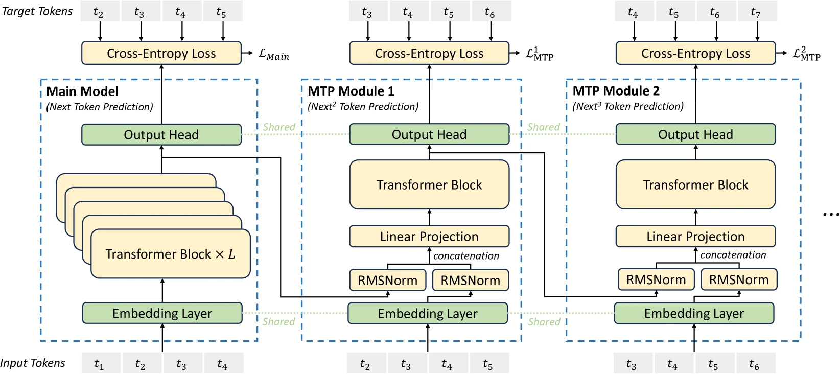
figure2: MTP implementation in DeepSeek, where they keep causal chain for prediction of each token at each depth
tl/dr: predict n-tokens at once, via shared trunk and n dedicated attention heads 14
Note that during inference, we only employ one attention head
Byte-Latent Transformer
idea: learn from raw-bytes and skip tokenizer/detokenizer protocol.
Feynman-Kac
Let V be the vocab of given transformers model, and S=V∗ the set of multi-token strings. Assume V contains token EOS and write F⊆S for the set of EOS-terminated strings.
Feynman-Kac Transformer model
is a tuple (s0,{Mt}t≥1,{Gt}t≥1) where:
s0∈S is an initial state, which will take as empty string ϵ
Mt(st∣st−1,fθ) is a Markov kernel from st−1∈Fc to st∈S, parameterised by a transformer network fθ:Fc→R∣V∣ mapping non-EOS-terminated strings to vectors of logits
Gt(st−1,st,fθ) is a potential function, mapping a pair (st−1,st)∈Fc×S to a real-valued non-negative score.
Goal: generate from distribution P that reweights Markov chain M by potential functions Gt. We define step-t filtering posteriors:
Note that we refer to standard sampling to methods such as argmax, top-k, nucleus, temperatures, et al., albeit each have a different ways to process logits.
We will consider these as standard sampling from an adjusted distribution↩
Rejection sampling follows a iterative sampling procedure that might looks superficially similar to speculative sampling:
Sample x∼q(x) and returns r∼U(0,1)
If r<Mq(x)p(x) return x
then go to 1
Where M=maxxq(x)p(x)
We could employ non-iterative version of rejection sampling instead of speculative sampling here (go through step 1 and 2, and otherwise sample an unmodifiedp(x) directly)
less efficient, given that the accept probability here is:
Ex∼q(x)Mq(x)p(x)=x∑p(x)x′minp(x′)q(x′)≤x∑p(x)min(1,p(x)q(x))=x∑min(p(x),q(x))
A lenience parameter l∈[0,1] to introduce further trade-off. This is useful when the distributions of draft models does not match the target model exactly.
this relies on q is sampled from this given distributions, and l increases α
In the case of greedy decoding (temperature=0), the draft essentially outputs xq′=argmaxq(x), so scaling lq(x) becomes a no-op, given that the argmax will be unchanged in this case. ↩
On Correctness of Speculative Sampling (SpS)
We will show that ∀p(x) and q(x), tokens sampled via speculative sampling from p(x) and q(x) are distributed identically to those sampled from p(x) alone.
also known as elapsed real time. This is different from CPU time, given that it measure the actual time taken from the start of the computer program, where as CPU time only measures time during which processor is actively working on a certain task or process↩
Denote the cost of running single steps of Mp by T.
Each run will then costs Tcγ+T=T(cγ+1) (running Mqγ times and running Mp once)
Given (1) procduces 1−α1−αγ+1 tokens
The cost to produces a token with speculative sampling would be 1−αγ+1(cγ+1)(1−α)T
Denote by T^ the number of arithmetic operations done by standard decoding per tokens, therefore speculative sampling costs T^c^γ+T^(γ+1) operations. Then divided by the expected tokens we got the desired results ↩
Gloeckle et al. (2024) employs n=4. The order of the forward and backward in a n-token prediction model with n=4 heads of the shared trunk works as follow:
z = model.shared(x)d = z.detach()d.requires_grad = Falsefor i in range(n): p = model.heads[i](d) loss(p, y[i]).backward()z.backward()
Chen, C., Borgeaud, S., Irving, G., Lespiau, J.-B., Sifre, L., & Jumper, J. (2023). Accelerating Large Language Model Decoding with Speculative Sampling. arXiv preprint arXiv:2302.01318 [arXiv]
Gao, X., Xie, W., Xiang, Y., & Ji, F. (2025). Falcon: Faster and Parallel Inference of Large Language Models through Enhanced Semi-Autoregressive Drafting and Custom-Designed Decoding Tree. arXiv preprint arXiv:2412.12639 [arXiv]
Leviathan, Y., Kalman, M., & Matias, Y. (2023). Fast Inference from Transformers via Speculative Decoding. arXiv preprint arXiv:2211.17192 [arXiv]
Li, Y., Wei, F., Zhang, C., & Zhang, H. (2024). EAGLE-2: Faster Inference of Language Models with Dynamic Draft Trees. arXiv preprint arXiv:2406.16858 [arXiv]
Li, Y., Wei, F., Zhang, C., & Zhang, H. (2025b). EAGLE-3: Scaling up Inference Acceleration of Large Language Models via Training-Time Test. arXiv preprint arXiv:2503.01840 [arXiv]
Liu, X., Daniel, C., Hu, L., Kwon, W., Li, Z., Mo, X., Cheung, A., Deng, Z., Stoica, I., & Zhang, H. (2024). Optimizing Speculative Decoding for Serving Large Language Models Using Goodput. arXiv preprint arXiv:2406.14066 [arXiv]
Mamou, J., Pereg, O., Korat, D., Berchansky, M., Timor, N., Wasserblat, M., & Schwartz, R. (2024). Dynamic Speculation Lookahead Accelerates Speculative Decoding of Large Language Models. arXiv preprint arXiv:2405.04304 [arXiv]
Stern, M., Shazeer, N., & Uszkoreit, J. (2018). Blockwise Parallel Decoding for Deep Autoregressive Models. arXiv preprint arXiv:1811.03115 [arXiv]
Wertheimer, D., Rosenkranz, J., Parnell, T., Suneja, S., Ranganathan, P., Ganti, R., & Srivatsa, M. (2024). Accelerating Production LLMs with Combined Token/Embedding Speculators. arXiv preprint arXiv:2404.19124 [arXiv]
Zhang, L., Wang, X., Huang, Y., & Xu, R. (2025). Learning Harmonized Representations for Speculative Sampling. arXiv preprint arXiv:2408.15766 [arXiv]
Zhou, Y., Lyu, K., Rawat, A. S., Menon, A. K., Rostamizadeh, A., Kumar, S., Kagy, J.-F., & Agarwal, R. (2024). DistillSpec: Improving Speculative Decoding via Knowledge Distillation. arXiv preprint arXiv:2310.08461 [arXiv]
Gholami, A., Yao, Z., Kim, S., Hooper, C., Mahoney, M. W., & Keutzer, K. (2024). AI and Memory Wall. arXiv preprint arXiv:2403.14123 [arXiv]
Gloeckle, F., Idrissi, B. Y., Rozière, B., Lopez-Paz, D., & Synnaeve, G. (2024). Better & Faster Large Language Models via Multi-token Prediction. arXiv preprint arXiv:2404.19737 [arXiv]
Lew, A. K., Zhi-Xuan, T., Grand, G., & Mansinghka, V. K. (2023). Sequential Monte Carlo Steering of Large Language Models using Probabilistic Programs. arXiv preprint arXiv:2306.03081 [arXiv]
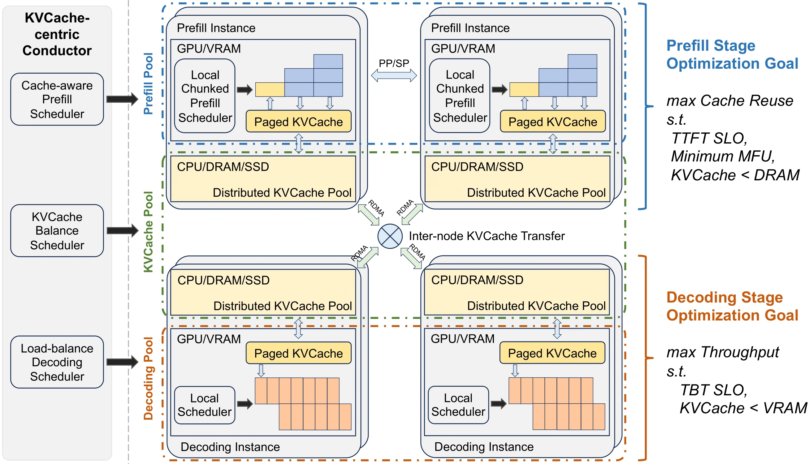
Qin, R., Li, Z., He, W., Zhang, M., Wu, Y., Zheng, W., & Xu, X. (2024). Mooncake: A KVCache-centric Disaggregated Architecture for LLM Serving. arXiv preprint arXiv:2407.00079 [arXiv]
Tay, Y., Dehghani, M., Bahri, D., & Metzler, D. (2022). Efficient Transformers: A Survey. arXiv preprint arXiv:2009.06732 [arXiv]
Vaswani, A., Shazeer, N., Parmar, N., Uszkoreit, J., Jones, L., Gomez, A. N., Kaiser, L., & Polosukhin, I. (2023). Attention Is All You Need. arXiv preprint arXiv:1706.03762 [arXiv]
 (Tay et al., 2022) in attention layers within information-dense data
(Li et al., 2025)
 . This is different from CPU time, given that it measure the actual time taken from the start of the computer program, where as CPU time only measures time during which processor is actively working on a certain task or process ↩