See also refresh on SQL and indexes with views, or this slides on SQL DSL, and final review
closure of
For a set of FDs , then closure is the set of all FDs that can be derived from
not to be confused with closure of an attribute set
rules
Lien vers l'original
Rule Description Reflexivity If , then Augmentation If , then for any Transitivity If and , then Union If and , then Decomposition If , then and
closure test
Given attribute set and FD set , we have is the closure of relative to
Or set of all FDs given/implied by
Steps:
Lien vers l'original
- Start:
- While there exists a s.t :
- End:
minimal basis
The idea is to remove redundant FDs.
for minimal cover for FDs
- Right sides are single attributes
- No FDs can be removed, otherwise is no longer a minimal basis
- No attribute can be removed from a LEFT SIDE
construction:
Lien vers l'original
- decompose RHS to single attributes
- repeatedly try to remove a FD to see if the remaining FDs are equivalent to the original set
- or is equivalent to
- repeatedly try to remove an attribute from LHS to see if the removed attribute can be derived from the remaining FDs.
Design theory
Keys
is a key if uniquely determines all of and no subset of does
K is a superkey for relation if contains a key of
see also: keys
functional dependency
Think of it as ” holds in ”
convention: no braces used for set of attributes, just instead of
properties
- splitting/combining
- trival FDs
- Armstrong’s Axioms
FD are generalisation of keys
superkey: , must include all the attributes of the relation on RHS
trivial
always hold (right side is a subset)
splitting/combining right side of FDs
when each of , , …, holds for
ex: is equiv to and
ex: and can be written as
Armstrong’s Axioms
Given are sets of attributes
rules
Rule Description Reflexivity If , then Augmentation If , then for any Transitivity If and , then Union If and , then Decomposition If , then and dependency inference
is implied by
transitivity
example: Key
List all the keys of with the following FDs:
sol:
closure test
Given attribute set and FD set , we have is the closure of relative to
Or set of all FDs given/implied by
Steps:
- Start:
- While there exists a s.t :
- End:
minimal basis
The idea is to remove redundant FDs.
for minimal cover for FDs
- Right sides are single attributes
- No FDs can be removed, otherwise is no longer a minimal basis
- No attribute can be removed from a LEFT SIDE
construction:
- decompose RHS to single attributes
- repeatedly try to remove a FD to see if the remaining FDs are equivalent to the original set
- or is equivalent to
- repeatedly try to remove an attribute from LHS to see if the removed attribute can be derived from the remaining FDs.
Schema decomposition
goal: avoid redundancy and minimize anomalies (update and deletion) w/o losing information
One can also think of projecting FDs as geometric projections within a given FDs space
good properties to have
- lossless join decomposition (should be able to reconstruct after decomposed)
- avoid anomalies (redundant data)
- preservation:
information loss with decomposition
- Decompose into and
- consider FD with and
- FD loss
- Attribute and not in the same relation (thus must join and to enforce , which is expensive)
- Join loss
- neither nor is in
A lossy decomposition results in the reconstruction of components to include additional information that is not in the original constructions
how can we test for losslessness?
A binary decomposition of into and is lossless iff:
- is the
- is the
if form a superkey of either or , then decomposition of is lossless
Projection
- Starts with
- For each subset
- Compute
- For each attribute
- If in : add to
- Compute minimal basis of
Normal forms
Normal Form Definition Key Requirements Example of Violation How to Fix First Normal Form (1NF) All columns contain atomic values and there are no repeating groups. - Each cell holds a single value (atomicity)
- No repeating groups or arraysA column storing multiple phone numbers in a single cell (e.g., “123-4567, 234-5678”). Split the values into separate rows or columns so each cell is atomic. Second Normal Form (2NF) A 1NF table where every non-key attribute depends on the whole of a composite key. - Already in 1NF
- No partial dependencies on a composite primary keyA table with a composite primary key (e.g., StudentID, CourseID) where a non-key attribute (e.g., StudentName) depends only on StudentID. Move attributes that depend on only part of the key into a separate table. Third Normal Form (3NF) A 2NF table with no transitive dependencies. - Already in 2NF
- No transitive dependencies (non-key attributes depend only on the key, not on other non-key attributes)A table where AdvisorOffice depends on AdvisorName, which in turn depends on StudentID. Put attributes like AdvisorName and AdvisorOffice in a separate Advisor table keyed by AdvisorID. Boyce-Codd Normal Form (BCNF) A stronger version of 3NF where every determinant is a candidate key. - For every functional dependency X → Y, X must be a candidate key A table where Professor → Course but Professor is not a candidate key. Decompose the table so that every functional dependency has a candidate key as its determinant. 1NF
no multi-valued attributes allowed
idea: think of storing a list of a values in an attributes
counter:
Course(name, instructor, [student, email]*)2NF
non-key attributes depend on candidate keys
idea: consider non-key attribute , then there exists an FD s.t. and is a candidate key
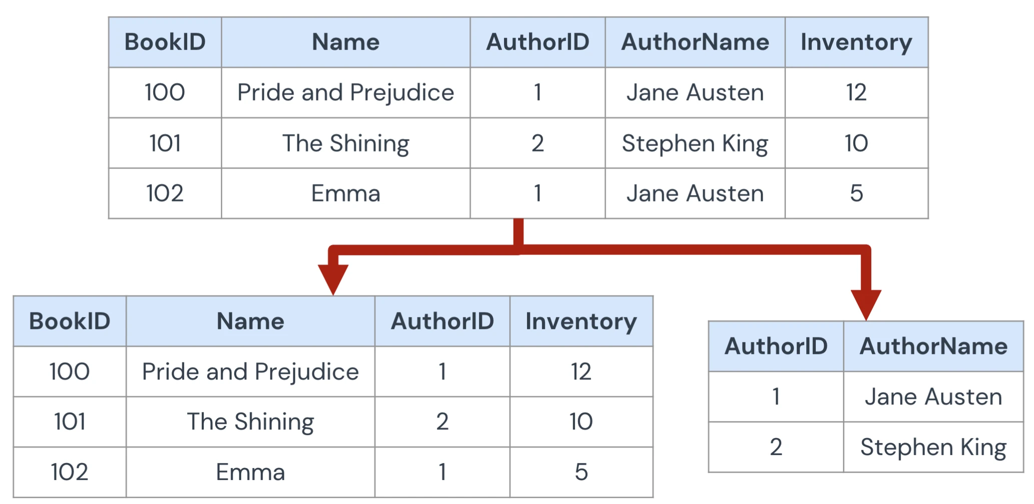
figure1: Second normal form, hwere AuthorName is dependent on AuthorID 3NF
non-prime attribute depend only on candidate keys
idea: consider FD , then either is a superkey, or is prime (part of a key)
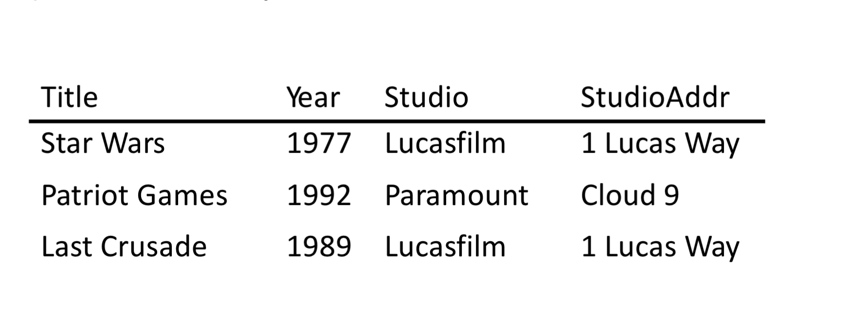
counter: , where
studioAddrdepends onstudiowhich is not a candidate keyfigure2: Three normal form counter example 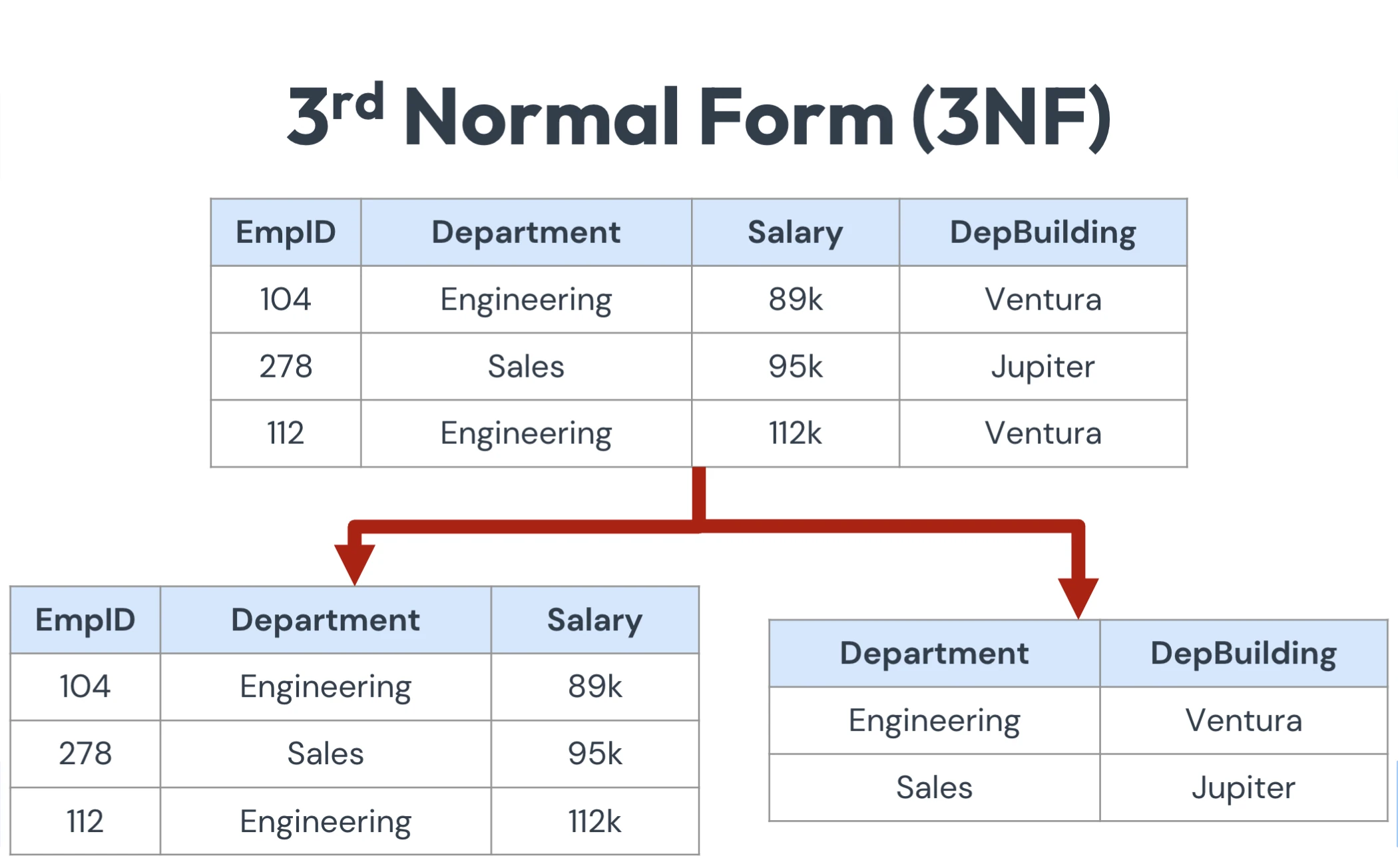
theorem
It is always possible to convert a schema to lossless join, dependency-preserving 3NF
what you get from 3NF
- Lossless join
- dependency preservation
- anomalies (doesn’t guarantee)
Boyce-Codd normal form (BCNF)
on additional restriction over 3NF where all non-trivial FDs have superkey LHS
theorem
We say a relation is in BCNF if is a non-trivial FD that holds in , and is a superkey 1
what you get from BCNF
- no dependency preservation (all original FDs should be satisfied)
- no anomalies
- Lossless join
decomposition into BCNF
relation with FDs , look for a BCNF violation ( is not a superkey)
Lien vers l'original
- Compute
- find ( is a superkey)
- Replace by relations with
- Continue to recursively decompose the two new relations
- Project given FDs onto the two new relations.
Relational Algebra
Operator Operation Example Selection Projection Cross-Product Natural Join Theta Join Rename Eliminate Duplicates Sort Tuples Grouping & Aggregation selection
idea: picking certain row
is the condition refers to attribute in
def: is all those tuples of that satisfies C
projection
idea: picking certain column
is the list of attributes from
products
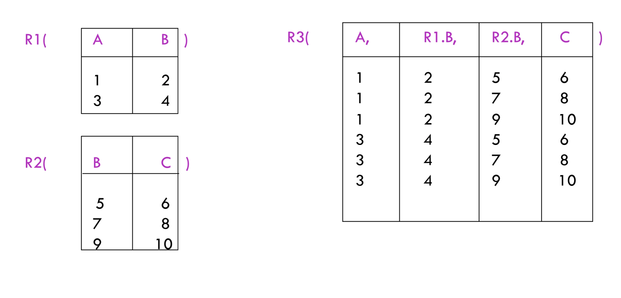
theta-join
idea: product of and then apply to results
think of where
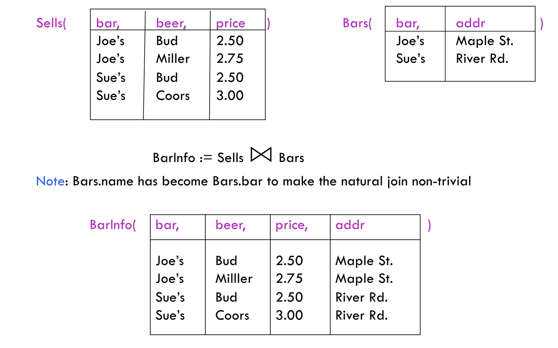
natural join
- equating attributes of the same name
- projecting out one copy of each pair of equated attributes
renaming
set operators
union compatible
two relations are said to be union compatible if they have the same set of attributes and types (domain) of the attributes are the same
i.e:
Student(sNumber, sName)andCourse(cNumber, cName)are not union compatiblebags
definition
modification of a set that allows repetition of elements
Think of is a bags, whereas is also considered a bag.
Lien vers l'originalin a sense, happens to also be a set.
Set Operations on Relations
For relations and that are union compatible, here’s how many times a tuple appears in the result:
Operation Symbol Result (occurrences of tuple ) Union Intersection Difference where is the number of times appears in and is the number of times it appears in .
sequence of assignments
precedence of relational operators:
expression tree
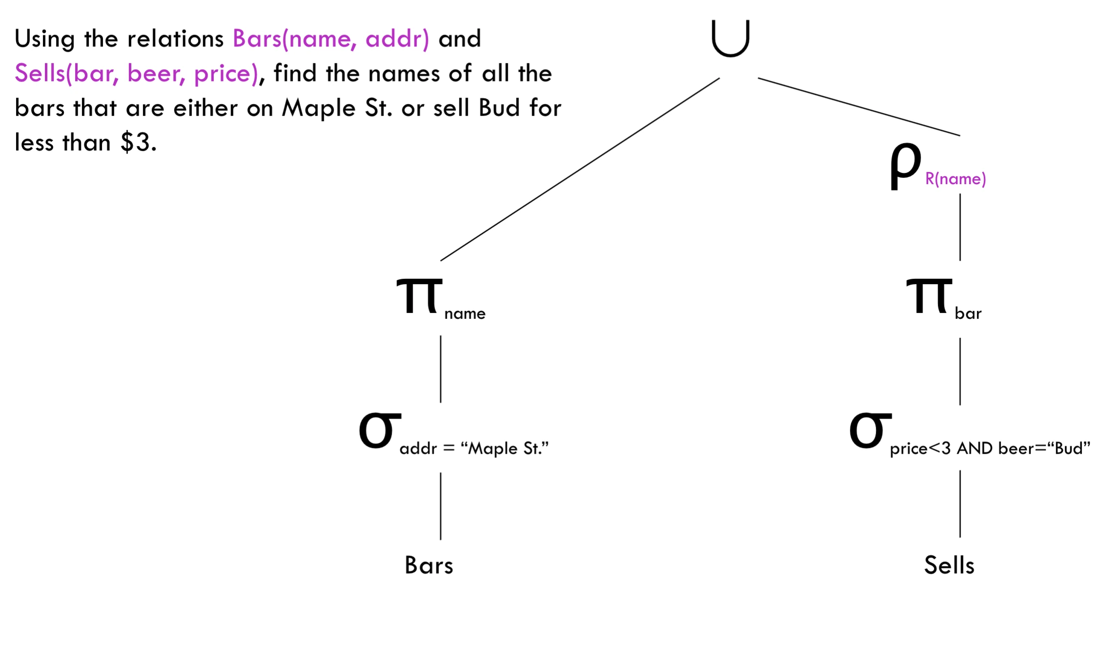
extended algebra
: eliminate duplication from bags
: sort tuples
grouping and aggregation
outerjoin: avoid dangling tuples
duplicate elimination
Think of it as converting it to set
sorting
with is a list of some attributes of
basically for ascending order, for descending order then use
applying aggregation
or
group accordingly to all grouping attributes on
per group, compute
AGG(A)for each aggrgation onresult has one tuple for each group: grouping attributes and aggregations
aggregation is applied to an entire column to produce a single results
outerjoin
essentially padding missing attributes with
NULLbag operations
remember that bag and set operations are different
set union is idempotent, whereas bags union is not.rightarrow
bag union:
bag intersection:
bag difference:
Lien vers l'original
Transaction
see also concurrency
A sequence of read/write
concurrency
inter-leaved processing: concurrent exec is interleaved within a single CPU.
parallel processing: process are concurrently executed on multiple CPUs.
source code ACID
- atomic: either performed in its entirety (DBMS’s responsibility)
- consistency: must take database from consistent state to
- isolation: appear as if they are being executed in isolation
- durability: changes applied must persist, even in the events of failure
Schedule
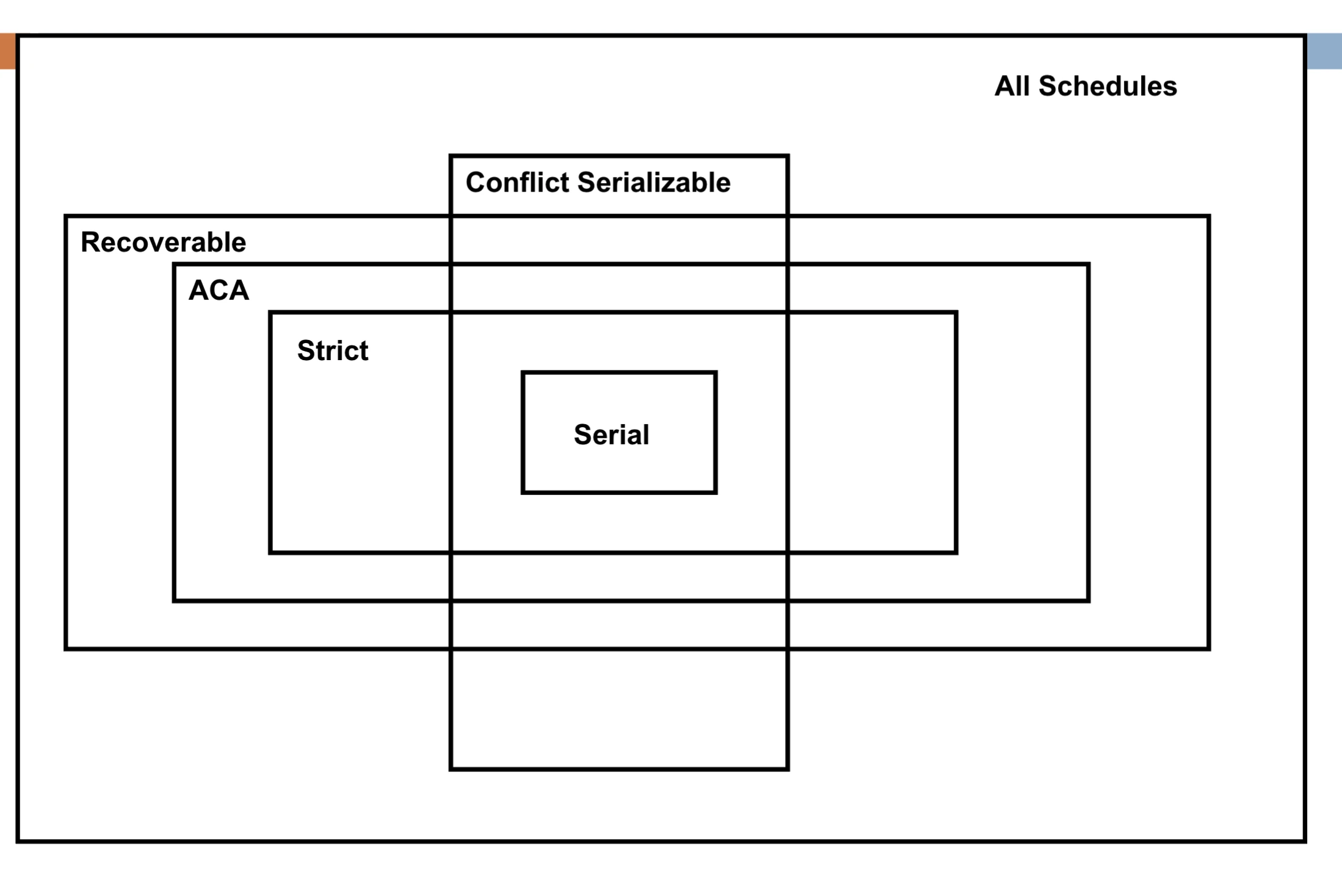
figure1: Venn diagram for schedule definition
a schedule of transaction is an ordering of operations of the transactions subject to the constrain that
For all transaction that participates in , the operations of in must appear in the same order in which they occur in
For example:
- serial schedule: does not interleave the actions of different transactions
- equivalent schedule: effect of executing any schedule are the same
serialisable schedule
a schedule that is equvalent to some serial execution of the set of committed transactions
serial
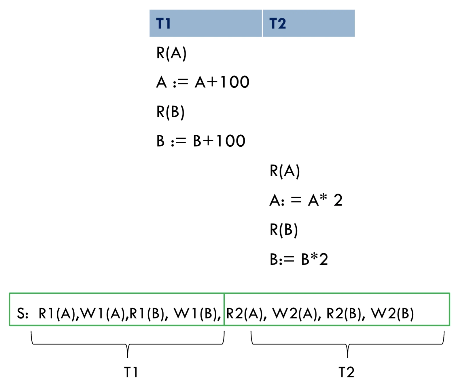
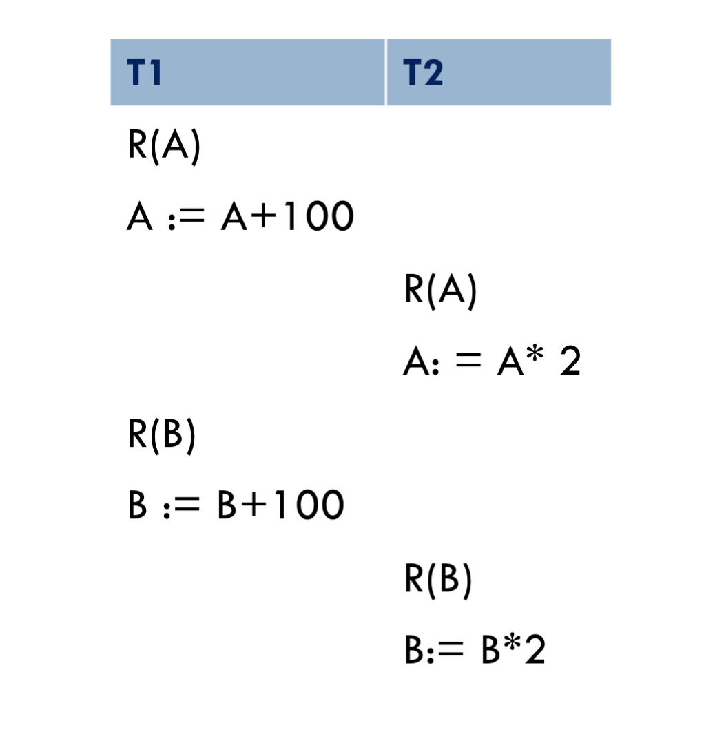
serialisable schedule
figure2: Note that this is not a serial schedule, given there are interleaved operations.
conflict
operations in schedule
said to be in conflict if they satisfy all of the following:
- belong to different operations
- access the same item
- at least one of the operations is a
write(A)
Concurrency Issue Description Annotation Dirty Read Reading uncommitted data WR Unrepeatable Read T2 changes item that was previously read by T1, while T1 is still in progress RW Lost Update T2 overwrites item while T1 is still in progress, causing T1’s changes to be lost WW conflict serialisable schedules
Two schedules are conflict equivalent if:
- involves the same actions of the same transaction
- every pair of conflicting actions is ordered the same way
Schedule is conflict serialisable if is conflict equivalent to some serial schedule
If two schedule and are conflict equivalent then they have the same effect by swapping non-conflicting ops
Every conflict serialisable schedule is serialisable
on conflict serialisable
only consider committed transaction
schedule with abort
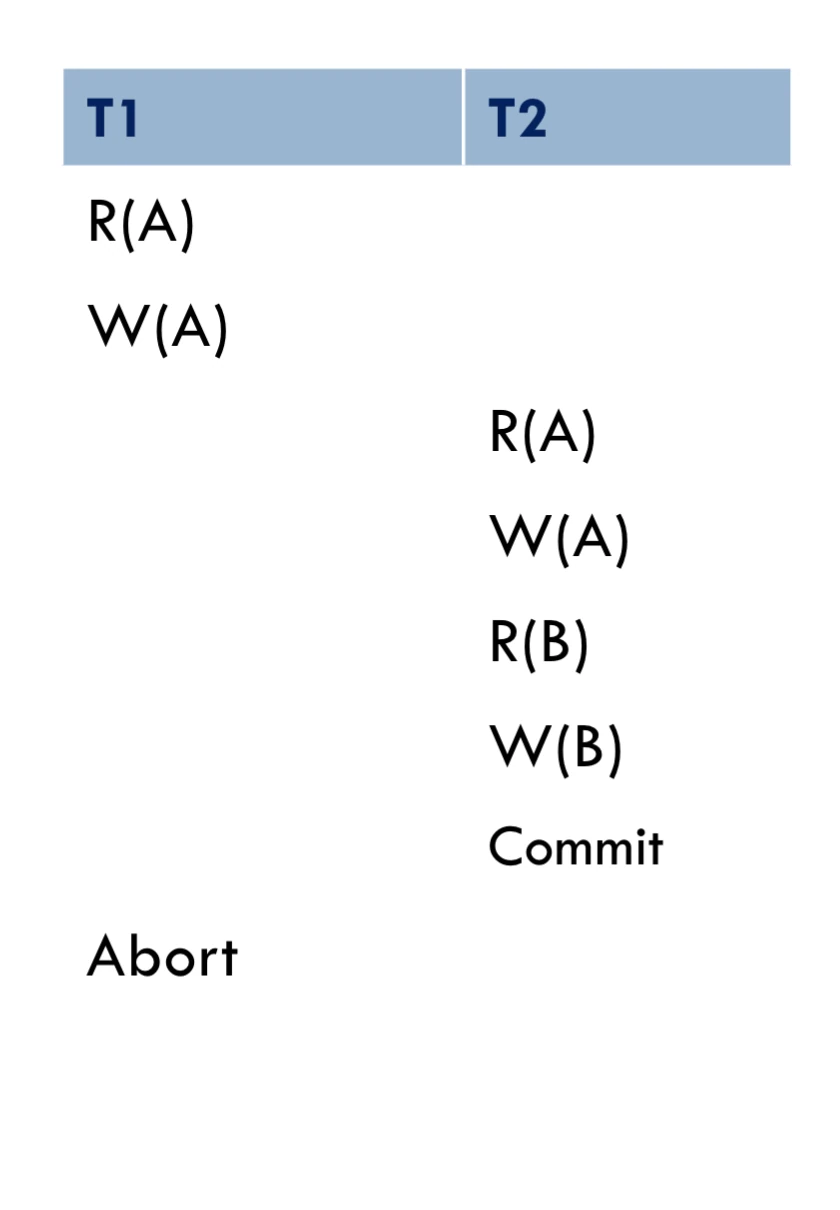
figure3: Note that this schedule is unrecoverable if T2 committed However, if T2 did not commit, we abort T1 and cascade to T2
need to avoid cascading abort
- if writes an object, then can read this only after commits
recoverable and avoid cascading aborts
Recoverable: a commits only after all it depends on commits.
ACA: idea of aborting a can be done without cascading the abort to other
ACA implies recoverable, not vice versa
precedent graph test
is a schedule conflict-serialisable?
- build a graph of all transactions
- Edge from to if comes first, and makes an action that conflicts with one of
if graphs has no cycle then it is conflict-serialisable
strict
if a value written by is not read or overwritten by another until abort/commit
Are recoverable and ACA
Lock-based concurrency control
think of mutex or a lock mechanism to control access to a data object
transaction must release the lock
notation
Li(A)means acquires lock for A, where asUi(A)releases lock for A
Lock Type None S X None OK OK OK S OK OK Conflict X OK Conflict Conflict lock compatibility matrix
overhead due to delays from blocking; minimize throughput
- use smallest sized object
- reduce time hold locks
- reduce hotspot
shared locks
for reading
exclusive lock
for write/read
strict two phase locking (Strict 2PL)
- Each must obtain a S lock on object before reading, and an X lock on object before writing
- All lock held by transaction will be released when transaction is completed
only schedule those precedence graph is acyclic
recoverable and ACA
Example:
T1 T2 L(A); R(A), W(A) L(A); DENIED... L(B); R(B), W(B) U(A), U(B) Commit; ...GRANTED R(A), W(A) L(B); R(B), W(B) U(A), U(B) Commit; implication
- only allow safe interleavings of transactions
- and access different objects, then no conflict and each may proceed
- serial action
two phase locking (2PL)
lax version of strict 2PL, where it allow to release locks before the end
- a transaction cannot request additional lock once it releases any lock
implication
- all lock requests must precede all unlock request
- ensure conflict serialisability
- two phase transaction growing phase, (or obtains lock) and shrinking phase (or release locks)
isolation
Isolation Level Description READ UNCOMMITTEDNo read-lock READ COMMITTEDShort duration read locks REPEATABLE READLong duration read/lock on individual items SERIALIZABLEAll locks long durations Deadlock
cycle of transactions waiting for locks to be released by each other
usually create a wait-for graph to detect cyclic actions
Lien vers l'original
wait-die: lower transactions never wait for higher priority transactions
wound-wait: is higher priority than then is aborted and restarts later with same timestamp, otherwise waits
